Installation

System requirements: Windows 10, ArcGIS Pro v2.2.4 or higher, License for Spatial Analyst extension if analysis of raster data is required

XLUR uses a number of Python modules/packages; however, most of these are Python base modules or are pre-installed with ArcGIS Pro (see the repository for a list of the required packages). Only four additional packages need to be installed. In ArcGIS Pro this can be done using the Python Package Manager. Follow these steps to install additional Python packages:

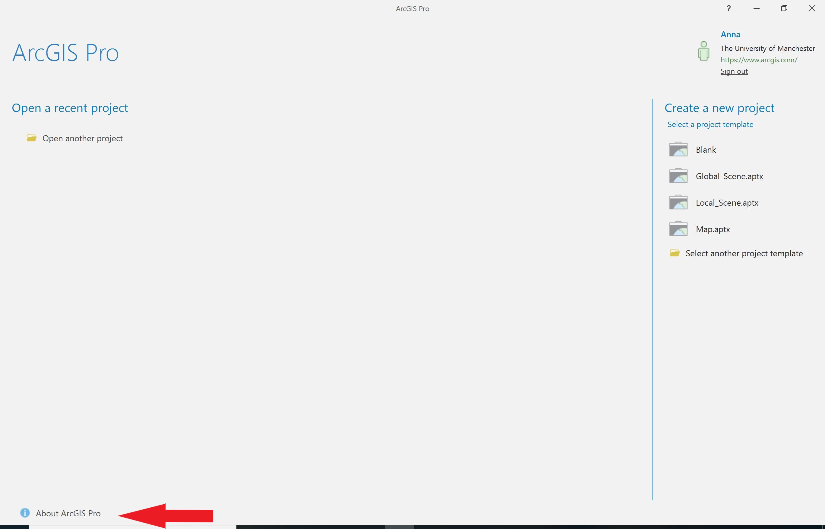
Open ArcGIS Pro. Click the About ArcGIS Pro button in the bottom left corner (denoted by the red arrow in the screenshot below). In ArcGIS Pro v.2.3 this button is called Settings.

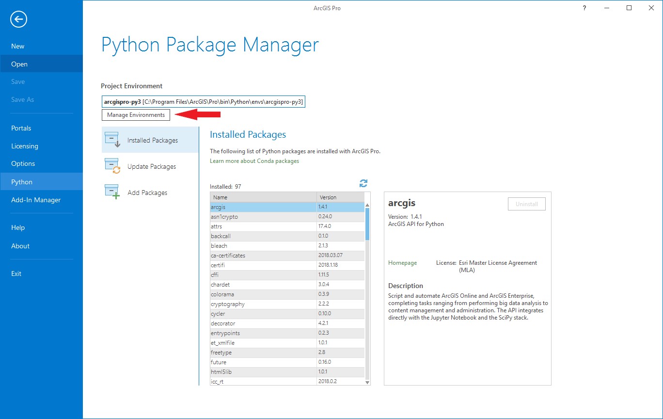
In the menu on the left hand side click Python. This will open the Python Package Manager. Click the Manage Environments button.

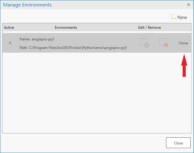
This will open the Manage Environments window. Since additional packages cannot be installed in the default environment, you will need to clone the default environment. Ensure that the default environment is selected (this is typically called ‘arcgispro-py3’), then click clone.

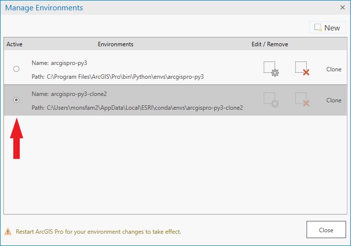
Creating the cloned environment may take a while, a blue line at the bottom of the window indicates that the process is still running. Once the clone has been created, click the radio button to make it the active environment. Click Close, then Exit ArcGIS Pro and restart it for the changes to take effect.

Restart ArcGIS Pro, click on About ArcGIS Pro, then click on Python in the menu on the left hand side. Under Project Environment you should see the name of the cloned environment. If you do not see the name of the cloned environment, repeat step 3 being careful not to exit the programme until the clone has been created. Click Add Packages.

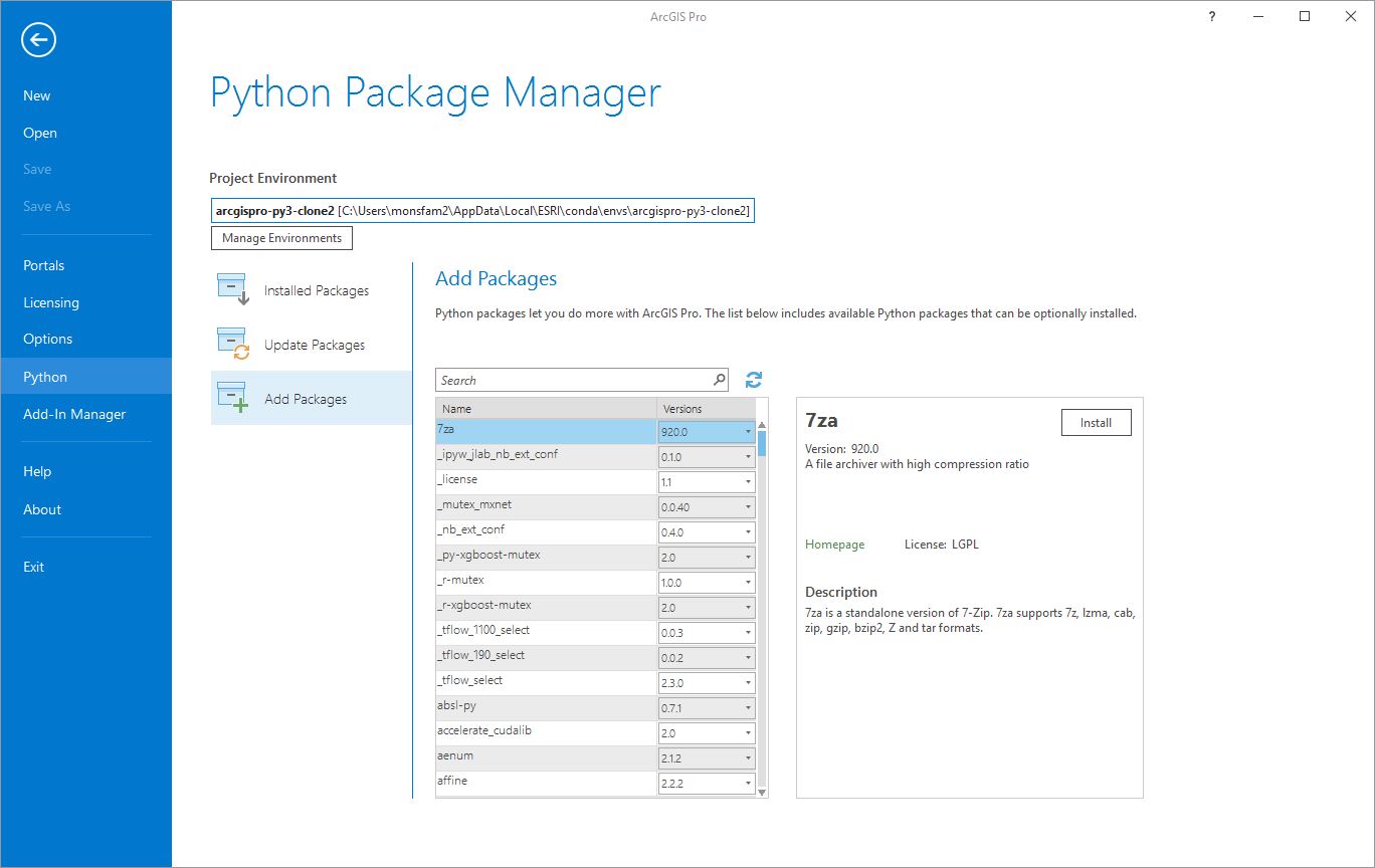
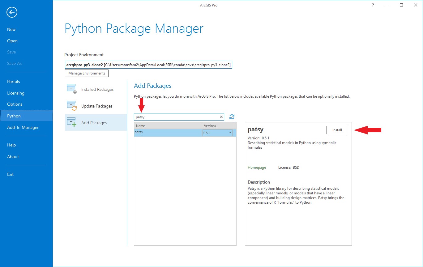
This opens the Add Packages interface. In the Search box type patsy. The patsy package should appear in the list below. Select the patsy package and click Install.

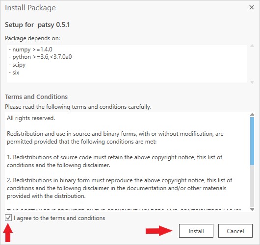
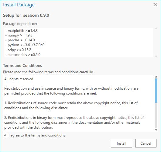
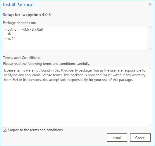
This will open the Install Package window. Tick the box in the bottom left to agree to the terms and conditions, then click Install.

The installation may take a while. Once the installation is finished, the list underneath Add Packages will refresh. If you scroll down the list, you will see that patsy is no longer on it (because it has been installed). If you want to check that the package has been installed, click on Installed Packages. If you scroll down the list of installed packages, patsy should be listed.

Repeat step 4 for the following packages:

statsmodels

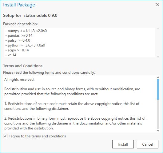
seaborn

wxpython

If you are planning to use raster data in your analysis, click on Licensing in the menu on the left hand side. Under Esri Extensions check that Spatial Analyst is licensed.
Click the back arrow in the menu on the left hand side. Click Open another project, browse to the XLUR.aprx ArcGIS Pro Project file and double-click to open it. The XLUR.aprx file can be found in the XLUR folder in the XLUR repository. In the Catalog window double-click Toolboxes, then double-click XLUR.tbx. This will open the XLUR toolbox, which contains the BuildLUR and ApplyLUR scripts. Running either of these script will open the Build LUR or Apply LUR wizard, respectively.

General Information

What is LUR?

Classic LUR

Land use regression (LUR) is a statistical method, which uses geospatial data to develop prediction models in environmental sciences. It is predominantly used in air pollution research to predict pollutant concentrations empirically within a given a study area. However, it has also been used for other environmental phenomena such as noise, air temperature and water microbiology.

The underlying principle of LUR is that a measured quantity (e.g. pollutant concentration, noise level, temperature etc) at a given location depends on characteristics of the surrounding environment, in particular on the presence and absence of sources and sinks, which increase and decrease values respectively.

LUR models are developed by using measured data from a number of monitoring sites as the dependent variable and data on the surrounding environment extracted as potential predictor variables in a multiple linear regression analysis. For example, in an air pollution study particulate matter concentrations might be measured at fifty monitoring sites. Then for each monitoring site potential predictor variables are extracted such as the area of industrial land use around the monitoring site, the distance to the nearest road, the number of motor vehicles on the nearest road etc. The particulate matter concentrations and the potential predictors are entered into a supervised machine learning process, which will try to construct a parsimonious multiple linear regression model. This model can then be used to predict particulate matter concentrations at any point within the study area.

The supervised machine learning process is based on the methodology used in the European Study of Cohorts for Air Pollution Effects (ESCAPE), which can be downloaded from http://www.escapeproject.eu/manuals/ESCAPE_Exposure-manualv9.pdf (a copy can be found in the Documentation folder). The ESCAPE exposure manual provides a detailed description of the steps required to construct a parsimonious multiple linear regression model; therefore, only a brief summary is presented here:

Prior to the statistical analysis a positive or negative direction of effect is assigned to each potential predictor variable by the user based on a priori knowledge of the subject area.
Using the dependent variable univariate linear regression models are created for each potential predictor variable. The linear regression models are ranked by their adjusted R² value. The model with the highest adjusted R² and in which the coefficient of the predictor variable matches the assigned direction of effect (see previous step) is selected as the starting model.
The remaining potential predictor variables are added to the starting model one by one. The new linear regression models are ranked by by their adjusted R² value. The model with the highest adjusted R² and in which the coefficients of all predictor variables match the assigned direction of effects is selected. If the adjusted R² of this model has increased by more than 1% compared to the previous model, it is used as the new model. If not, the variable selection process stops and the previous model is used as the intermediate model. Using these selection criteria potential predictor variables are added to the model until the increase in adjusted R² becomes less than 1% or until no potential predictor variables are left. The resulting model is the intermedite model.
The predictor variables included in the intermediate model are inspected. If all predictor variables are statistically significant (p<0.1), the intermediate model becomes the final model. If non-significant (p>0.1) predictors are present in the intermediate model, predictor variables are removed from the intermediate model until all predictor variables are statistically significant and their coefficients still match the assigned direction of effect. The resulting model will become the final model.

XLUR will provide a range of diagnosics for the final model which can be used to further analyse the suitability and robustness of the final model.

Hybrid LUR

Hybrid models can also be developed. Hybrid models in XLUR are based on an extension of the ESCAPE methodology developed by de Hoogh et al. (see https://doi.org/10.1016/j.envres.2016.07.005). In the XLUR tool a hybrid model is a model in which one or more mandatory variables are selected by the user. These mandatory variables are forced into the model prior to the starting model, regardless of the amount of variance that they explain or their direction of effect. Once the mandatory variables have been entered potential predictor variables are added and models are selected in the same way as described for the Classic LUR model. It should be noted that mandatory variables will not be removed during step 4 described above. They will remain in the model regardless of their sigficance level.

An example of this would be using the output from dispersion models run at a coarse spatial resolution as a mandatory variable, which could add a measure of global variability to the measures of local variability used in LUR.

The XLUR Wizard

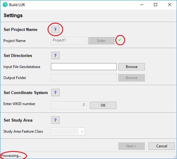
The XLUR wizard guides the user through building and applying LUR models from within the ArcGIS software. The user must complete each input field in the wizard starting at the top of the page and then moving downwards. The statusbar at the bottom of wizard indicates if an input field is ready for an entry or if it is currently being processed. Some inputs may take a while to be processed. Once an input has been completed a green tick mark will appear next to it. Clicking on the question mark button next to each section heading will open a help window with further information on how to complete each section. The user may exit the wizard at any time by clicking on the Cancel button; however, all progress made in the wizard will be lost.

The wizard window can be resized by dragging the sides or by clicking on the maximise button in the title bar.

There are three types of windows that may appear during the process of completing the wizard.

Information Windows

Information windows simply confirm a choice made by the user. They are non-critical.

Warning Windows

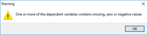
A warning window highlights a potential problem in the dataset selected by the user. This problem may be critical or non-critical and it is up to the user to decide whether to proceed.

Error Windows

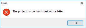
An error window indicates that an incorrect entry has been made into an input field, that an invalid selection has been made or that a dataset has a critical problem. This is a critical problem and needs to be addressed before proceeding with the wizard. In some cases, for example if the dataset has a critical problem, the user may need to exit the wizard, address the problem and then start afresh.

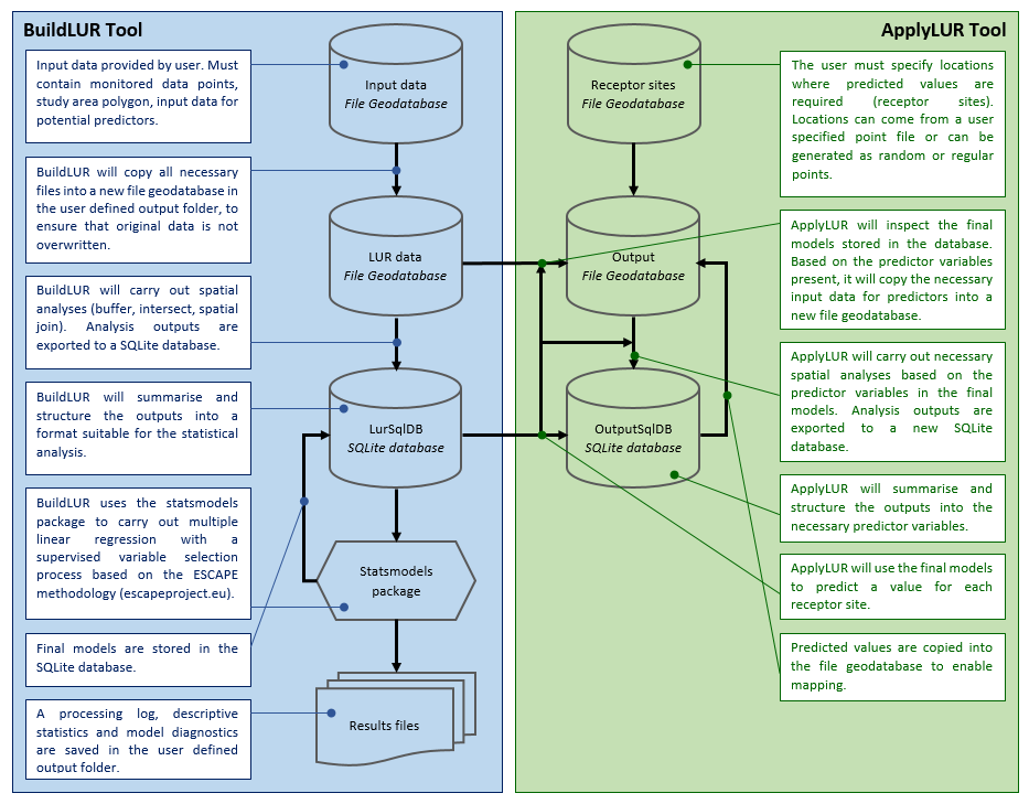
How does XLUR work?

XLUR is written in Python. It consists of two script tools, BuildLUR and ApplyLUR, which are stored in the XLUR toolbox in the XLUR project. The diagram below provides an overview of the architecture and process flow associated with each tool.

Data Preparation

It is essential to prepare the data carefully prior to using XLUR. XLUR will carry out some very basic checks of the data, i.e. it will check that features are located within the study area and if necessary display a warning message. XLUR will not clean or prepare the data for use in the BuildLUR wizard. Users should carefully check all feature classes and raster files that they intend to use. In particular, feature classes should be checked for spatial duplicates (e.g. using the Find Identical and Delete Identical tools) and invalid geometries (e.g. using the Check Geometry and Repair Geometry tools).

To be used by the BuildLUR tool all feature classes and raster files must be stored in the same File Geodatabase.

The following tabs show further information for different input datasets.

Study Area

The file geodatabase must contain a polygon feature class that represents the boundaries of the study area.

This feature class must contain:

exactly one feature, which as a minimum encompasses all of the monitoring sites.

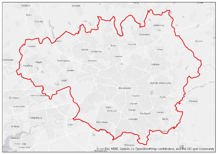
Typically, a feature class of administrative boundaries is used to define the study area. For example, the red polygon below shows the boundary of the Greater Manchester administrative area. If no such feature class is available, it can be created, either manually or by using the Minimum Bounding Geometry Tool.

Dependent Variable

The file geodatabase must contain a point feature class of the monitoring sites, which will be used as the dependent variable when building the LUR model. Each row in this feature class must be a unique location, i.e. there must be no spatial duplicates.

The point feature class must contain:

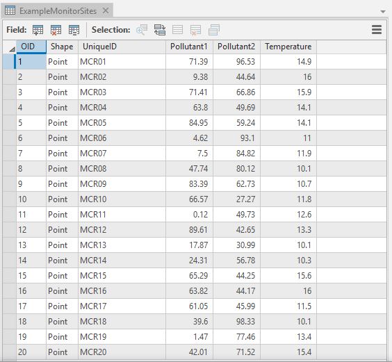
a text field with a unique identifier for each monitoring site.
one or more numeric fields with monitored values (e.g. pollutant concentrations, temperatures, bacterial counts).

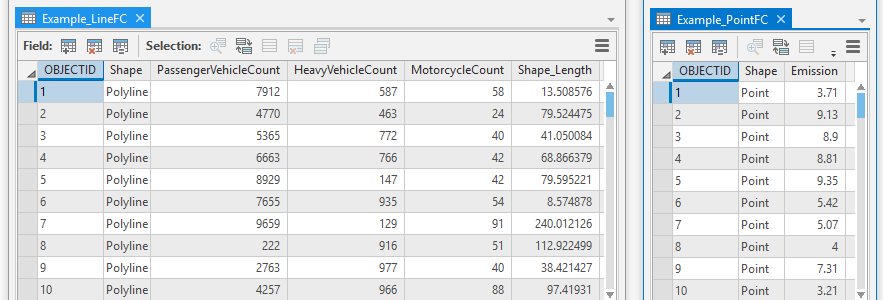
The table below shows an example of an attribute table of a monitoring sites feature class. The feature class may contain other fields. These will be ignored during the analysis, but they may slow down the performance of the XLUR tools.

Predictor Variables

Predictor variables can be derived from both vector data and raster data. Multiple predictor variables can be derived from a single vector dataset, depending on additional criteria such as the number of buffers, attribute categories and aggregation methods. In contrast, only a single predictor can be derived from a raster dataset. To build a LUR model, typically hundreds of potential predictor variables are extracted and then assessed in the statistical analysis. Technically, the BuildLUR tool can be run with only one predictor, but the resulting model will be very limited.

Vector maps

From vector data predictor variables can be extracted based on circular buffers around the monitoring sites or based on the distance to the nearest feature. Each of these methods can be applied to polygon, line or point vector data.

Buffer based Predictors

XLUR will draw one or more circular buffers around each monitoring site (the radius of the buffer is determined by the user). It will then use the Intersect tool to extract features and their associated attributes from a polygon, line or point feature class selected by the user. Geometric attributes are automatically recalculated.

This feature class must contain:

a text field which identifies the category that each feature belongs to. For example, a polygon feature class of land use would contain a text field that identifies which land use category (e.g. residential, commercial, industrial) each polygon feature belongs to. A road feature class would contain a text field that identifies the road type (e.g. motorway, primary, secondary) of each line feature. A tree feature class might contain a text field that shows the species of each point feature. The text of the category field will be used as part of the variable naming schema, for details of the name schema see Step 3 - Predictors. It is strongly recommended to only use alphanumeric characters in the text of the category field. Non-alphanumeric characters can cause problems and may stop XLUR from running. Please note that the BuildLUR tool will remove any whitespace and punctuation from the category field, before using it.

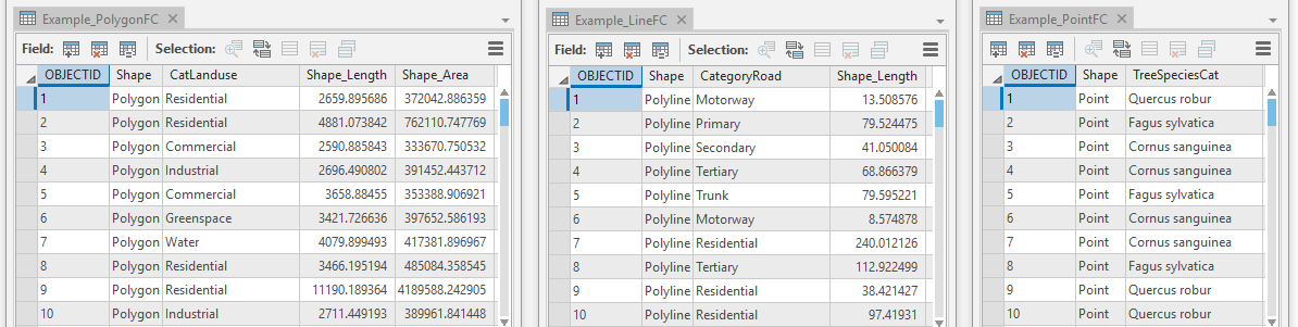
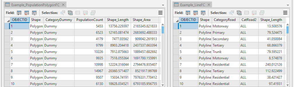
If the features of the feature class cannot be categorised, then a text field should be used in which all features have the same value. For example, a polygon feature class of population density would not need a category; therefore a “dummy” text field should be added with identical values. In a line feature class of roads it may also be useful to analyse all roads as well as roads by category, therefore to this feature class an additional text field could be added in which all fields are set to “all”. The tables below show some examples of “dummy” category fields.

The feature class may contain:

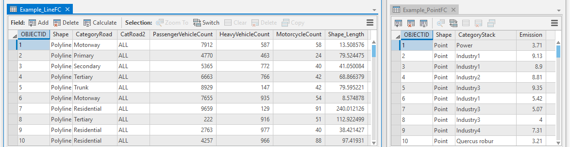
one or more numeric fields showing attribute values for each feature. If the chosen aggregation method is total area, total length or point count, a numeric field is not required. However, if the chosen aggregation method is area weighted value, area*value, length weighted value, length*value, sum of values, mean of values or median of values, then the feature class must contain at least one numeric field (see Build LUR Step 3 - Predictors for further information on aggregation methods). For example, a line feature class of roads may contain one or more fields showing traffic counts for each feature (line segment or row in the attribute table). A point feature class of chimney stacks may contain a field showing emission rates for each feature. The attribute tables below show some examples of value fields.

Distance based Predictors

XLUR will identify the nearest polygon, line or point feature to each monitoring site point location from a feature class selected by the user The nearest feature is based on the Euclidean (straight line) distance and is expressed in the map units defined by the coordinate system specified the BuildLUR tool. Depending on the chosen method it will calculate the distance to the nearest feature, provide the value of an attribute of the nearest feature (e.g. traffic flow) or calculate a combination of these two.

The feature class may contain:

one or more numeric fields showing attribute values for each feature. If the chosen method is distance, inverse distance or inverse distance squared, then a numeric field is not required. However, if the chosen method is value, value*distance, value*inverse distance or value*inverse distance squared, then the feature class must contain at least one numeric field. For example, a line feature class of roads may contain one or more fields showing traffic counts for each feature (line segment or row in attribute table). A point feature class of chimney stacks may contain a field showing emission rates for each feature. The attribute tables below show some examples of value fields.

Raster maps

From raster data only the value of the raster cell that is spatially coincident with the monitoring site point can be extracted. Since standard raster grids can only hold one value per cell, no table schema is required.

Build LUR

To create a new LUR model double-click the BuildLUR script in the XLUR toolbox. The BuildLUR tool will appear in the Geoprocessing pane. Click the Run button in the bottom right corner to run the tool.

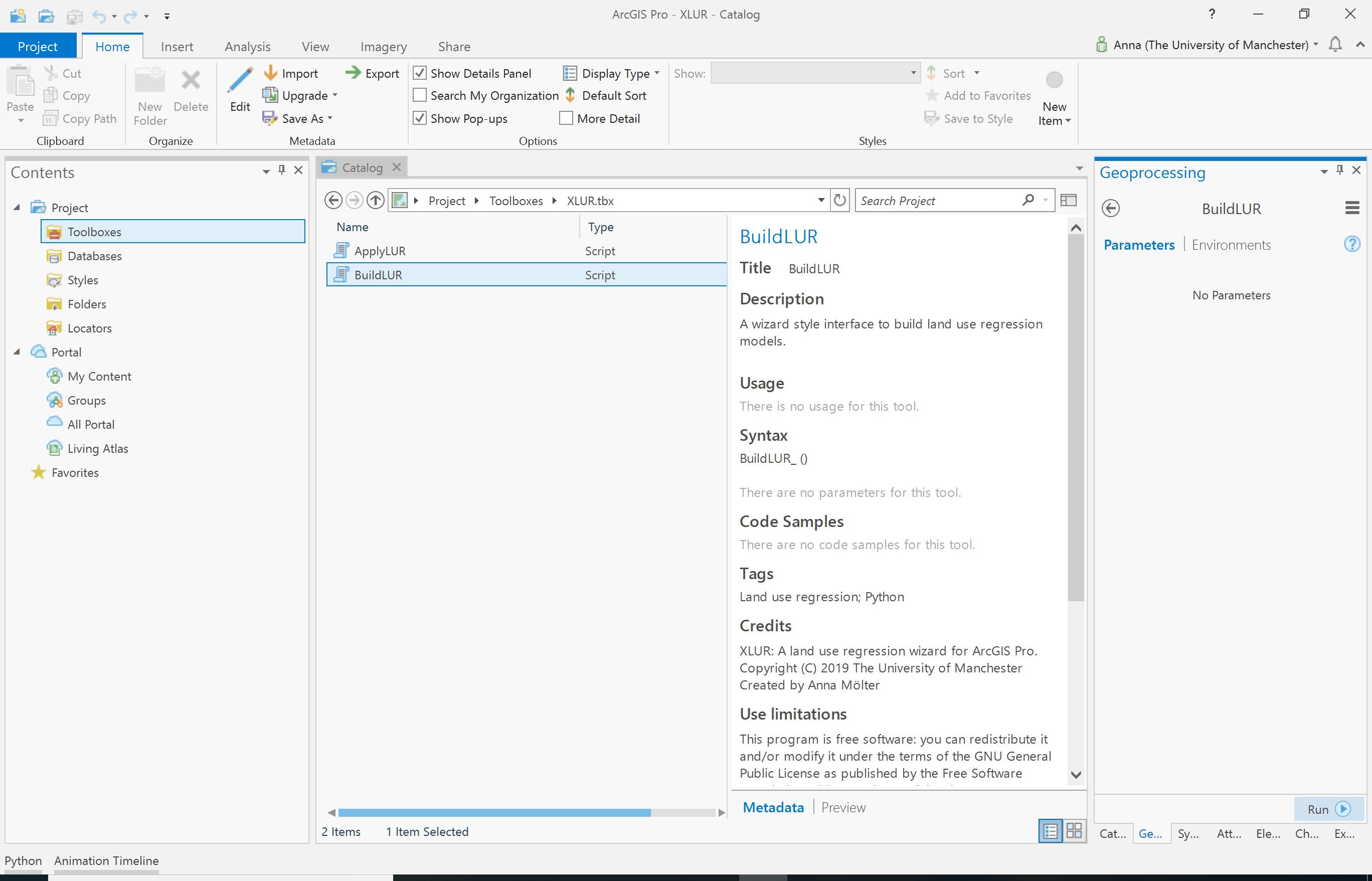
This will open the BuildLUR wizard. The wizard will guide you through the process of creating a LUR model by using the following steps:

Step 1 - Settings

This step is required to specify some general settings to build a LUR model.

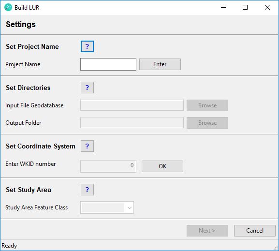
Set Project Name

XLUR Wizard

Set Project Name

Project Name

Type in a name for your LUR project. The name must have a length of at least 1 character and can have a maximum length of 10 characters. The name can contain text (ISO basic Latin alphabet), numbers and underscores. The name must start with a text character.

Click the Enter button to continue.

Set Directories

XLUR Wizard

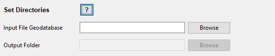
Set Directories

Input File Geodatabase

Click on the Browse button to open the directory dialog. Navigate to the file geodatabase containing your data. This must be a folder with a '.gdb' extension.

Click on the file geodatabase, then click the Select Folder button. The file path to the input file geodatabase and a green tick mark will appear. Depending on the size of the file geodatabase this may take a while.

Output Folder

Click on the Browse button to open the directory dialog. Navigate to a folder where you would like to save your results. This folder must not have a '.gdb' extension. You must have write access to this folder. It is recommended to use a folder that has no spaces in its file path. Inside the folder a new folder will be created automatically by the Wizard. The name of this folder will be the project name that you have entered followed by a date and time stamp: [Project name]_[Date_Time]. Inside this folder a number of files will be created throughout the wizard:

File name	Description	Created during
[Project name]_[Date_Time].gdb	A file geodatabase containing the feature classes and raster files used to develop the LUR model	Settings
LurSqlDB.sqlite	A SQLite database containing intermediate and aggregated data for the statistical analysis	Settings
GOTCHA.txt	A text file containing errors caught during processing	Settings
LOG_[Date_Time].txt	A text file showing selections made in the wizard and the machine learning steps during the statistical analysis (if done via the wizard)	Settings
Descriptive_analyses_[Date_Time].pdf	A pdf of descriptive statistics of the outcome and predictor variables	Model
CorrelationMatrix_Vars_[Date_Time].csv	A comma separated text file showing a correlation matrix of all variables	Model
Diagnostic_plots_dep[Outcome variable]_[Date_Time].pdf	A pdf of diagnostic plots for the final model of the outcome variable	Model
LOOCV_dep[Outcome variable]_[Date_Time].pdf	A pdf of the leave one out cross validation plot	Model
Residuals.csv	A comma separated text file of the final model residuals	Model

Click on the folder, then click the Select Folder button. The file path to the folder and a green tick mark will appear. Depending on the size of the folder this may take a while.

Set Coordinate System

XLUR Wizard

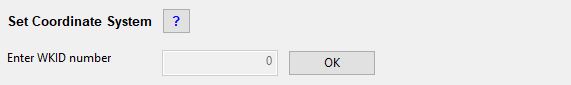
Set Coordinate System

Enter WKID number

The user must specify a projected coordinate system for the data. The wizard will automatically create a feature dataset called LURdata inside the [Project name]_[Date_Time].gdb file geodatabase. The specified coordinate system will be used as the spatial reference for the LURdata feature datatset. Feature classes selected during step 2 (Outcomes) and step 3 (Predictors) of the wizard will be imported into the LURdata feature dataset prior to analysis. This ensures that all feature classes used in the analysis have the same spatial reference. Raster files will be projected into the specified coordinate system prior to analysis, due to the fact that they cannot be imported into a feature dataset.

ESRI uses the Well-Known ID (WKID) to define the spatial reference. Use this link to find the WKID of the projected coordinate system of your choice. For example the British National Grid is WKID:27700.

Click the OK button. If a valid WKID has been entered, the name of the selected coordinate system will be shown. Click the OK button and a green tick mark will appear.

The unit of the coordinate system will determine the unit of the buffer distances. For example, if the coordinate system is defined in metres, then the buffer distances need to be specified in metres. If the coordinate system is defined in feet, then the buffer distances need to be specified in feet.

Set Study Area

XLUR Wizard

Set Study Area

Study Area Feature Class

From the dropdown menu select a polygon feature class that represents your study area. The feature class must contain exactly one feature. As a minimum the polygon area must encompass all of the monitoring sites.

If the input file geodatabase does not contain a study area polygon feature class, exit the wizard and create a study area feature class, for example by using the Minimum Bounding Geometry tool.

The feature class will be imported into the LURdata feature dataset. Once this step is complete a green tick mark will appear and the Next > button will be activated. This completes the Settings step.

Step 2 - Outcomes

In this step the dependent or outcome variables of the regression analysis are specified.

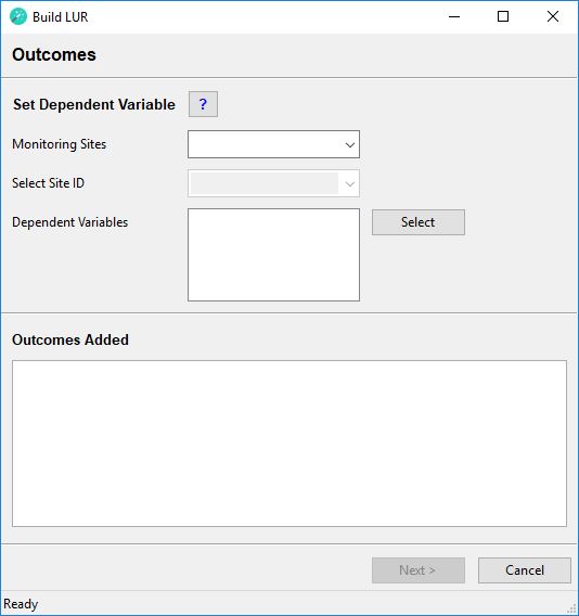
Set Dependent Variable

XLUR Wizard

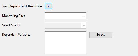
Set Dependent Variable

Monitoring Sites

From the dropdown menu select the point feature class containing the monitoring site locations (dependent variable). Each row (point) must be a unique location, i.e. there must be no spatial duplicates. The spatial extent of the monitoring site feature class must be smaller than and within the spatial extent of the study area.

The point feature class attribute table must contain a text field with IDs for the monitoring sites and one or more numeric fields with monitored data.

Select Site ID

From the dropdown menu select the text field, which shows IDs of the monitoring sites. The IDs must be unique and each point must have a value (i.e. the ID must not be missing). The wizard will automatically rename this field SiteID and add integer IDs to improve performance. However, model diagnostics will show the text IDs.

Dependent Variables

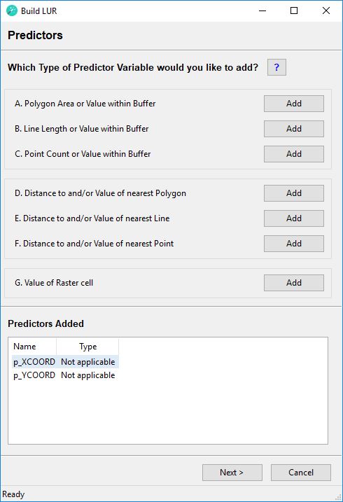
Tick all fields that contain monitored data and that you would like to develop a model for. These fields will be used as the dependent variable in the statistical analysis. Individual models will be developed for each dependent variable, i.e. if you tick more than one field, the corresponding number of models will be developed. Click the Select button. The selected feature class and fields will be imported into the LURdata feature dataset. Fields containing dependent variables will be automatically renamed using the following schema: dep[Original name of numeric field]. Predictor variables containing the X coordinate and Y coordinate of each site will be automatically added and will be called p_XCOORD and p_YCOORD.

If this step is completed successfully, a green tick mark will appear and the selected variables will appear under Outcomes Added. The Next > button will be activated. This completes the Outcomes step.

A warning message may appear, if the selected numeric fields for the dependent variable contain missing, zero or negative values. The user must decide whether this is acceptable or not. A minimum of 8 values is required for the statistical analysis.

Step 3 - Predictors

In this step the predictor or independent variables of the regression analysis are specified.

Predictor variables can be derived from vector data and from raster data. From vector data predictor variables can be extracted based on circular buffers around the monitoring site point locations or based on the distance to the nearest feature. Since vector data can be polygons, lines or points, this results in six possible types of predictor variables. From raster data only the value of the raster cell that is spatially coincident with the monitoring site point can be extracted, adding one more possible type of predictor. Therefore, in total seven types of predictor variables can be extracted and entered into the statistical analysis. Each type of variable can produce multiple predictors, depending on additional settings such as the number of buffer distances, the number of categories within a feature class, or the aggregation/extraction method specified.

Buffer based Predictors

Polygon Area or Value within Buffer

For this type of variable a polygon feature class should be used, which has a spatial extent that is larger than: the study area + the largest buffer distance. The polygon feature class should not contain duplicates or invalid geometries (if uncertain about invalid geometries, run the Repair Geometries tool prior to running the wizard). The polygon feature class must contain a text field, which identifies a category for each polygon. If the feature class contains only one category, a dummy text field should be created with all rows set to the same value.

Polygon Area within Buffer

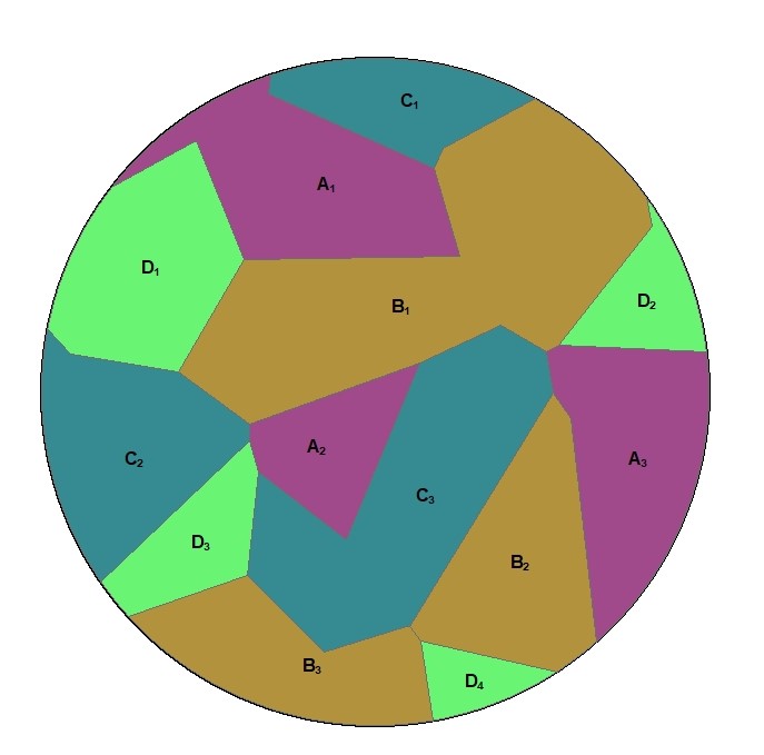
This example diagram is based on a polygon feature class with four categories (A,B,C,D). For a given buffer distance the wizard will calculate the total area (in the squared map unit of the projected coordinate system) of each category within the buffer, e.g.

Total area of category A = Area of A₁ + Area of A₂ + Area A₃
Total area of category B = Area of B₁ + Area of B₂ + Area B₃
Total area of category C = Area of C₁ + Area of C₂ + Area C₃
Total area of category D = Area of D₁ + Area of D₂ + Area D₃ + Area D₄

A real life example of this variable type would be a polygon feature class of land use. Each category would contain a different type of land use, for example residential, industrial, natural etc. Total land areas of each land use category within the circular buffer would be produced, e.g. in m² for the British National Grid.

Polygon Value within Buffer

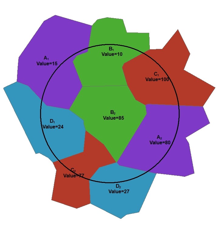
This example diagram is based on a polygon feature class with four categories (A,B,C,D) and each polygon has a numeric value attribute (“Value”). For a given buffer distance the wizard will calculate the total area weighted value for each category within the buffer, e.g.

Total area weighted value of category A = ((Area of A₁ inside buffer / Total Area of A₁) x Value of A₁) + ((Area of A₂ inside buffer / Total Area of A₂) x Value of A₂)
Total area weighted value of category B = ((Area of B₁ inside buffer / Total Area of B₁) x Value of B₁) + ((Area of B₂ inside buffer / Total Area of B₂) x Value of B₂)
Total area weighted value of category C = ((Area of C₁ inside buffer / Total Area of C₁) x Value of C₁) + ((Area of C₂ inside buffer / Total Area of C₂) x Value of C₂)
Total area weighted value of category D = ((Area of D₁ inside buffer / Total Area of D₁) x Value of D₁) + ((Area of D₂ inside buffer / Total Area of D₂) x Value of D₂)

A real life example of this variable type would be a polygon feature class of population density.

Alternatively, the wizard can calculate the total sum of the product of the polygon area and the polygon value, e.g.

Total sum of product of area and value of category A = (Area of A₁ inside buffer x Value of A₁) + (Area of A₂ inside buffer x Value of A₂)
Total sum of product of area and value of category B = (Area of B₁ inside buffer x Value of B₁) + (Area of B₂ inside buffer x Value of B₂)
Total sum of product of area and value of category C = (Area of C₁ inside buffer x Value of C₁) + (Area of C₂ inside buffer x Value of C₂)
Total sum of product of area and value of category D = (Area of D₁ inside buffer x Value of D₁) + (Area of D₂ inside buffer x Value of D₂)

A real life example of this variable type would be a polygon feature class of area emission sources such as fugitive emissions from land use categories based on different estimated car parking densities. Another example is anthropogenic heat emissions from different residential land uses depending on housing characteristics and estimated energy use.

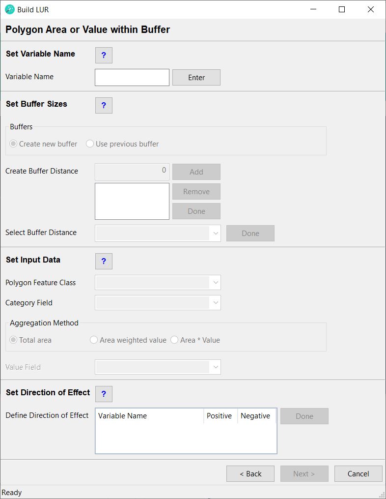
Set Variable Name

XLUR Wizard

Set Variable Name

Variable Name

Type in a name for the predictor variable to be created. This must be a unique name, i.e. the same name cannot be assigned to two or more different predictor variables. The name must have a length of at least 1 character and can have a maximum length of 20 characters (ISO basic Latin alphabet). The name cannot contain numbers, spaces or special characters. It is recommended to use a name that will help users to identify the input dataset that the predictor was derived from (e.g. use "landuse" rather than "PredictorOne"). Click the Enter button.

Name Schema for Polygon Area or Value within Buffer

Predictor variables extracted through this method will appear in the following name schema:

pA_[name entered by user]_[category name]_[buffer distance]_[aggregation method]

where:

pA - set automatically: p indicates that this is a predictor variable, A indicates the type of predictor variable. Click here to see a list of the possible types of predictor variables.
[name entered by user] - set by user: the variable name entered by the user.
[category name] - set automatically: the polygon feature class must contain a text field, which identifies a category for each polygon. This text field will be selected under Set Input Data. This part of the name schema identifies the category that the predictor variable belongs to. If the feature class contains only one category, a dummy text field should be created with all rows set to the same text string. This is the text string that would be shown in this part of the name.
[buffer distance] - set automatically: the buffer distance used to extract this variable. Buffer distances will be entered under Set Buffer Sizes.
[aggregation method] - set automatically: the method used to aggregate the extracted data:
- sum = sum of polygon area
- wtv = area weighted value
- mtv = area * value

Examples:

pA_landusearea_residential_500_sum - This predictor variable was extracted using a land use polygon feature class. The feature class contained a number of land use categories and this predictor contains the total area of residential land use within a 500m buffer

pA_popdensweighted_dummy_1000_wtv - This predictor variable was extracted using a feature class of population density polygons. This feature class contains only one category, therefore a dummy text field was created and all rows were set to the string "dummy". The naming schema shows that this predictor variable contains area weighted values within a 1000m buffer.

Set Buffer Sizes

XLUR Wizard

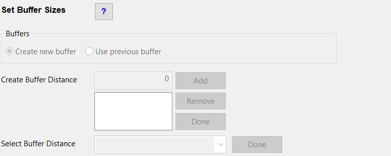
Set Buffer Sizes

Buffers

You can choose between creating a new set of one or more buffers or you can use a previous set of buffers.

If this is the first time in this Build LUR session that a buffer based predictor is created, then no previous buffers will be available, and you have to select Create new buffer. If you have already created a buffer based predictor during this Build LUR session, then you can re-use the buffers by selecting Use previous buffer.

Create Buffer Distance

Type in a buffer distance. The unit of the buffer distance is the same as the map unit of the projected coordinate system. Click the Add button. The buffer distance will be listed in the box. To add another buffer type in another buffer distance and click the Add button.

If a buffer distance is entered incorrectly, click on the incorrect distance to select it, then click the Remove button.

After all required buffer distances have been added, click the Done button. This will create a multiple ring buffer feature class in the LURdata feature dataset.

Select Buffer Distance

From the dropdown menu select the set of buffers that you would like to use again. Click on the set of buffers that you would like to use to ensure that it is selected. Then click the Done button.

Set Input Data

XLUR Wizard

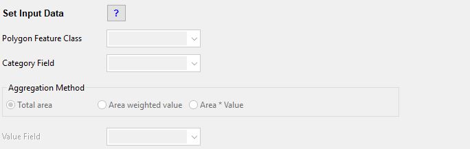
Set Input Data

Polygon Feature Class

From the dropdown menu select the polygon feature class from which you would like to extract data. The polygon feature class should have a spatial extent that is larger than: the study area + the largest buffer distance. The polygon feature class should not contain spatial duplicates or invalid geometries (if uncertain about invalid geometries, run the Check Geometry or Repair Geometry tool prior to running the wizard). The polygon feature class must contain a text field, which identifies a category for each polygon. If the feature class contains only one category, a dummy text field should be created with all rows set to the same text string. If the Area weighted value or Area * Value aggregation method will be used, the polygon feature class must also contain a numeric field.

Category Field

From the dropdown menu select the text field, which identifies the category of each polygon. If the feature class contains only one category, select a dummy text field in which all rows are set to the same text string.

Aggregation Method

Select the aggregation method to be used for this predictor variable.

Total area - This will calculate the sum of all polygon areas within each buffer and category. Click here for further details.
Area weighted value - This will calculate an area weighted value within each buffer and category. Click here for further details.
Area * Value - This will multiply the area of each polygon with a user selected value field. Click here for further details.

Value Field

From the dropdown menu select the numeric field to be used in the Area weighted value or Area * Value aggregation method. If this field contains missing data, then polygons with missing values may be extracted in the intersect analysis. Please be aware that the Area weighted value and Area * Value aggregation methods will ignore rows with missing data and the calculated value will be based on the non-missing data only. After a field has been selected a green tick mark will appear.

Set Direction of Effect

XLUR Wizard

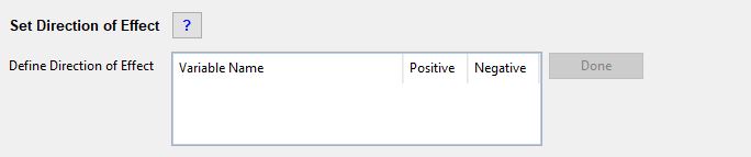
Set Direction of Effect

Define Direction of Effect

For each row in this box select whether the predictor variable is expected to have a positive or a negative direction of effect. The user has to make an a priori assumption for each predictor variable: a positive direction of effect is a predictor variable that will increase the value of the dependent variable, i.e. it is considered to be a source of the dependent variable and the beta coefficient is expected to be positive. A negative direction of effect is a predictor variable that will decrease the value of the dependent variable, i.e. it is considered to be a sink of the dependent variable and the beta coefficient is expected to be negative. These specifications will be used as model selection criteria in the statistical analysis; therefore, the user must consider carefully whether each predictor variable has a positive or a negative direction of effect. Incorrect specifications will lead to incorrect LUR models!

After all predictor variables in the list have been defined as either positive or negative, click the Done button. A green tick mark will appear and the Next > button will be activated. This completes this step. The newly created predictor variables will be listed in the Predictors Added box on the next page.

Line Length or Value within Buffer

For this type of variable a line feature class should be used, which has a spatial extent that is larger than: the study area + the largest buffer distance. The line feature class should not contain duplicates.The line feature class must contain a text field, which identifies a category for each line. If the feature class contains only one category, a dummy text field should be created with all rows set to the same value.

Line Length within Buffer

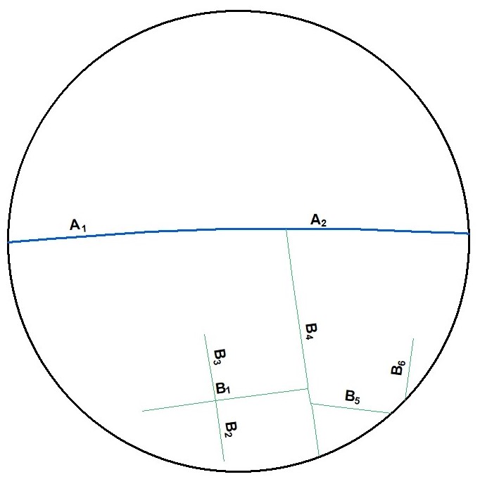
This example diagram is based on a line feature class with two categories (A,B). For a given buffer distance the wizard will calculate the total length (in the map unit of the projected coordinate system) of each category within the buffer, e.g.

Total length of category A = Length of A₁ + Length of A₂
Total length of category B = Length of B₁ + Length of B₂ + Length B₃ + Length B₄ + Length B₅ + Length B₆

A real life example of this variable type would be a line feature class of roads. Each category would contain a different type of road, for example motorway, local street etc. Total line lengths of each land use category within the circular buffer would be produced, e.g. in m for the British National Grid.

Line Value within Buffer

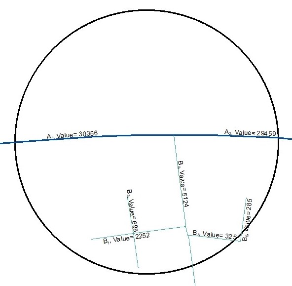
This example diagram is based on a line feature class with two categories (A,B) and each line has a numeric value. For a given buffer distance the wizard will calculate the total length weighted value for each category within the buffer, e.g.

Total length weighted value of category A = ((Length of A₁ inside buffer / Total Length of A₁) x Value of A₁) + ((Length of A₂ inside buffer / Total Length of A₂) x Value of A₂)
Total length weighted value of category B = ((Length of B₁ inside buffer / Total Length of B₁) x Value of B₁) + ((Length of B₂ inside buffer / Total Length of B₂) x Value of B₂) + ((Length of B₃ inside buffer / Total Length of B₃) x Value of B₃) + ((Length of B₄ inside buffer / Total Length of B₄) x Value of B₄) + ((Length of B₅ inside buffer / Total Length of B₅) x Value of B₅) + ((Length of B₆ inside buffer / Total Length of B₆) x Value of B₆)

A real life example of this variable type would be a line feature class of traffic counts.

Alternatively, the wizard can calculate the total sum of the product of the line length and the line value, e.g.

Total sum of product of length and value of category A = (Length of A₁ inside buffer x Value of A₁) + (Length of A₂ inside buffer x Value of A₂)
Total sum of product of length and value of category B = (Length of B₁ inside buffer x Value of B₁) + (Length of B₂ inside buffer x Value of B₂) + (Length of B₃ inside buffer x Value of B₃) + (Length of B₄ inside buffer x Value of B₄) + (Length of B₅ inside buffer x Value of B₅) + (Length of B₆ inside buffer x Value of B₆)

A real life example of this variable type would be a line feature class of proxy emissions loadings represented by average vehicle-kilometres per day.

Set Variable Name

XLUR Wizard

Set Variable Name

Variable Name

Type in a name for the predictor variable to be created. This must be a unique name, i.e. the same name cannot be assigned to two or more different predictor variables. The name must have a length of at least 1 character and can have a maximum length of 20 characters (ISO basic Latin alphabet). The name cannot contain numbers, spaces or special characters. It is recommended to use a name that will help users to identify the input dataset that the predictor was derived from (e.g. use "roads" rather than "PredictorOne"). Click the Enter button.

Name Schema for Line Length or Value within Buffer

Predictor variables extracted through this method will appear in the following name schema:

pB_[name entered by user]_[category name]_[buffer distance]_[aggregation method]

where:

pA - set automatically: p indicates that this is a predictor variable, B indicates the type of predictor variable. Click here to see a list of the possible types of predictor variables.
[name entered by user] - set by user: the variable name entered by the user.
[category name] - set automatically: the line feature class must contain a text field, which identifies a category for each line. This text field will be selected under Set Input Data. This part of the name schema identifies the category that the predictor variable belongs to. If the feature class contains only one category, a dummy text field should be created with all rows set to the same text string. This is the text string that would be shown in this part of the name.
[buffer distance] - set automatically: the buffer distance used to extract this variable. Buffer distances will be entered under Set Buffer Sizes.
[aggregation method] - set automatically: the method used to aggregate the extracted data:
- sum = sum of line lengths
- wtv = length weighted value
- mtv = length * value

Examples:

pB_roadlenth_motorway_500_sum - This predictor variable was extracted using a line feature class of roads. The feature class contained a number of road categories and this predictor contains the total length of motorway within a 500m buffer

pB_roadlengthtraffic_major_1000_mtv - This predictor variable was extracted using a line feature class of roads with traffic counts. The naming schema shows that this predictor variable contains the length of major roads multiplied with the traffic count within a 1000m buffer.

Set Buffer Sizes

XLUR Wizard

Set Buffer Sizes

Buffers

You can choose between creating a new set of one or more buffers or you can use a previous set of buffers.

Create Buffer Distance

If a buffer distance is entered incorrectly, click on the incorrect distance to select it, then click the Remove button.

After all required buffer distances have been added, click the Done button. This will create a multiple ring buffer feature class in the LURdata feature dataset.

Select Buffer Distance

From the dropdown menu select the set of buffers that you would like to use again. Click on the set of buffers that you would like to use to ensure that it is selected. Then click the Done button.

Set Input Data

XLUR Wizard

Set Input Data

Line Feature Class

From the dropdown menu select the line feature class from which you would like to extract data. The line feature class should have a spatial extent that is larger than the study area and the largest buffer distance combined. The line feature class must contain a text field, which identifies a category for each line. If the feature class contains only one category, a dummy text field should be created with all rows set to the same text string. If the Length weighted value or Length * Value aggregation method will be used, the line feature class must also contain a numeric field.

Category Field

From the dropdown menu select the text field, which identifies the category of each line. If the feature class contains only one category, select a dummy text field in which all rows are set to the same text string.

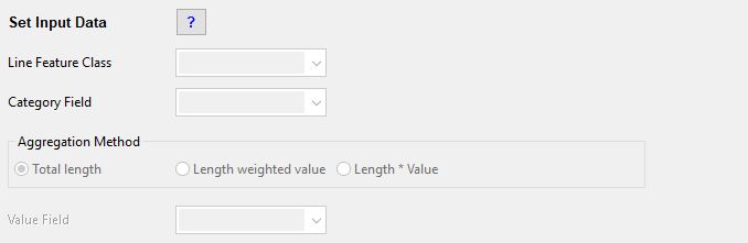
Aggregation Method

Select the aggregation method to be used for this predictor variable.

Total length - This will calculate the sum of all line lengths within each buffer and category. Click here for further details.
Length weighted value - This will calculate a length weighted value within each buffer and category. Click here for further details.
Length * Value - This will multiply the length of each polygon with a user selected value field. Click here for further details.

Value Field

From the dropdown menu select the numeric field to be used in the Length weighted value or Length * Value aggregation method. If this field contains missing data, then lines with missing values may be extracted in the intersect analysis. Please be aware that the Length weighted value and Length * Value aggregation methods will ignore rows with missing data and the calculated value will be based on the non-missing data only. After a field has been selected a green tick mark will appear.

Set Direction of Effect

XLUR Wizard

Set Direction of Effect

Define Direction of Effect

Point Count or Value within Buffer

For this type of variable a point feature class should be used, which has a spatial extent that is larger than: the study area + the largest buffer distance. The point feature class should not contain duplicates. The point feature class must contain a text field, which identifies a category for each point. If the feature class contains only one category, a dummy text field should be created with all rows set to the same value.

Point Count within Buffer

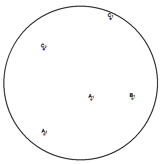
This example diagram is based on a point feature class with three categories (A,B,C). For a given buffer distance the wizard will count the number of points belonging to each category within the buffer, e.g.

Total count of category A = {A₁, A₂}
Total count of category B = {B₁ }
Total count of category C = {C₁, C₂}

A real life example of this variable type would be a point feature class of trees. Each category would contain a different tree species, for example Quercus robur, Fagus sylvatica, Cornus sanguinea etc.The count would therefore be the number of individuals of each species within the buffer. Another example would be the count of particular stacks (chimneys) used as a proxy of emission rates.

Point Value within Buffer

This example diagram is based on a point feature class with three categories (A,B,C) and each point has a numeric value. For a given buffer distance the wizard will calculate the sum of values for each category within the buffer, e.g.

Sum of values of category A = Value of A₁ + Value of A₂
Sum of values of category B = Value of B₁
Sum of values of category C = Value of C₁ + Value of C₂

A real life example of this variable type would be a point feature class of chimney stacks with different emission rates (e.g. grammes of NOx per hour).

Alternatively, the wizard can calculate the mean or median of the values, e.g.

Mean of values of category A = (Value of A₁ + Value of A₂) / Number of points within buffer belonging to category A
Mean of values of category B = Value of B₁ / Number of points within buffer belonging to category B
Mean of values of category C = (Value of C₁ + Value of C) / Number of points within buffer belonging to category C₂

A real life example of this variable type would be tree height.

Set Variable Name

XLUR Wizard

Set Variable Name

Variable Name

Type in a name for the predictor variable to be created. This must be a unique name, i.e. the same name cannot be assigned to two or more different predictor variables. The name must have a length of at least 1 character and can have a maximum length of 20 characters (ISO basic Latin alphabet). The name cannot contain numbers, spaces or special characters. It is recommended to use a name that will help users to identify the input dataset that the predictor was derived from (e.g. use "chimneys" rather than "PredictorOne"). Click the Enter button.

Name Schema for Point Count or Value within Buffer

Predictor variables extracted through this method will appear in the following name schema:

pC_[name entered by user]_[category name]_[buffer distance]_[aggregation method]

where:

pC - set automatically: p indicates that this is a predictor variable, C indicates the type of predictor variable. Click here to see a list of the possible types of predictor variables.
[name entered by user] - set by user: the variable name entered by the user.
[category name] - set automatically: the point feature class must contain a text field, which identifies a category for each point. This text field will be selected under Set Input Data. This part of the name schema identifies the category that the predictor variable belongs to. If the feature class contains only one category, a dummy text field should be created with all rows set to the same text string. This is the text string that would be shown in this part of the name.
[buffer distance] - set automatically: the buffer distance used to extract this variable. Buffer distances will be entered under Set Buffer Sizes.
[aggregation method] - set automatically: the method used to aggregate the extracted data:
- num = the number of points within the buffer
- sum = the sum of point values within the buffer
- avg = the mean of the point values
- med = the median of the point values

Examples:

pC_chimneycount_industrial_500_num - This predictor variable was extracted using a point feature class of chimney stacks. The feature class contained a number of building categories and this predictor contains the number of industrial chimney stacks within a 500m buffer

pC_emissionmedian_dummy_1000_med - This predictor variable was extracted using a point feature class of chimney stacks with emission rates. This feature class contains only one category, therefore a dummy text field was created and all rows were set to the string "dummy". The naming schema shows that this predictor variable contains the median emission rate from all chimney stacks within a 1000m buffer.

Set Buffer Sizes

XLUR Wizard

Set Buffer Sizes

Buffers

You can choose between creating a new set of one or more buffers or you can use a previous set of buffers.

Create Buffer Distance

If a buffer distance is entered incorrectly, click on the incorrect distance to select it, then click the Remove button.

After all required buffer distances have been added, click the Done button. This will create a multiple ring buffer feature class in the LURdata feature dataset.

Select Buffer Distance

From the dropdown menu select the set of buffers that you would like to use again. Click on the set of buffers that you would like to use to ensure that it is selected. Then click the Done button.

Set Input Data

XLUR Wizard

Set Input Data

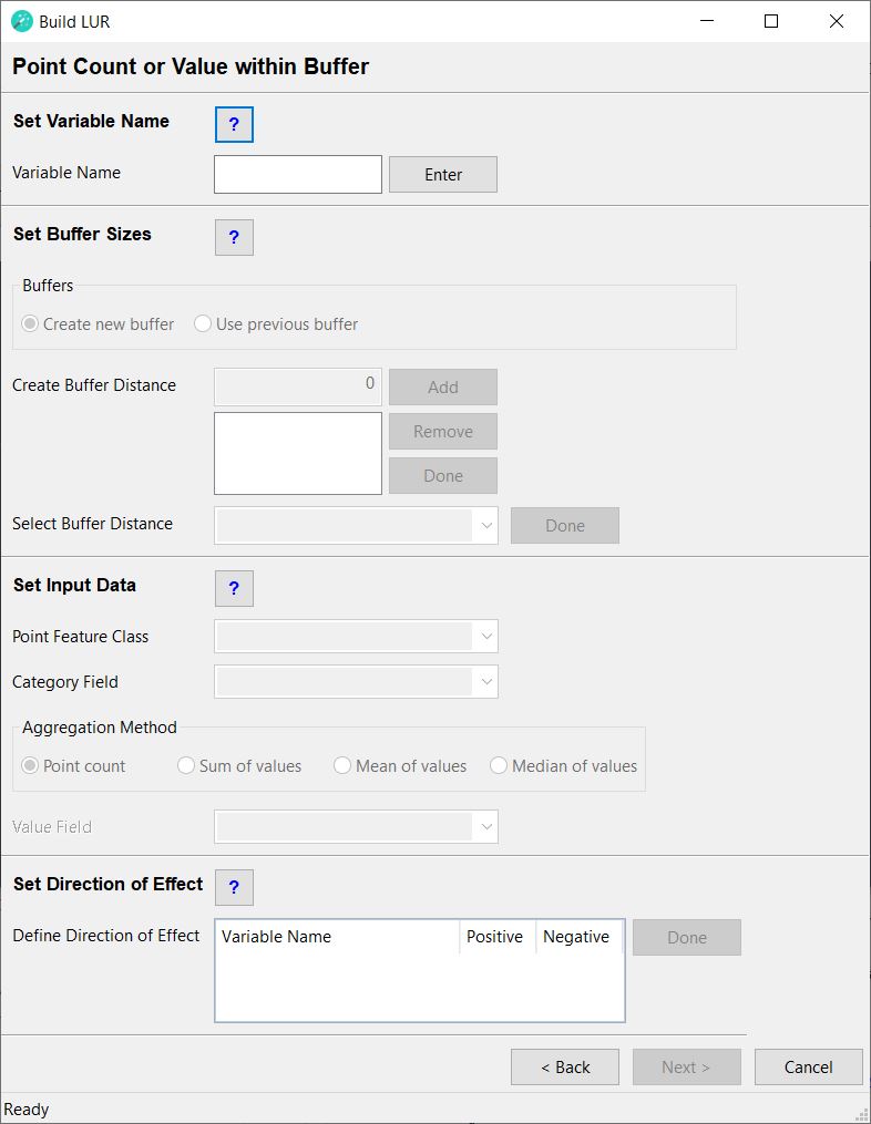
Point Feature Class

From the dropdown menu select the point feature class from which you would like to extract data. The point feature class should have a spatial extent that is larger than the study area and the largest buffer distance combined. The point feature class must contain a text field, which identifies a category for each point. If the feature class contains only one category, a dummy text field should be created with all rows set to the same text string. If the Sum of values, Mean of values or Median of values aggregation method will be used, the point feature class must also contain a numeric field.

Category Field

From the dropdown menu select the text field, which identifies the category of each point. If the feature class contains only one category, select a dummy text field in which all rows are set to the same text string.

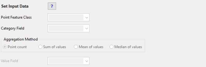
Aggregation Method

Select the aggregation method to be used for this predictor variable.

Point count - This will count the points within each buffer and category. Click here for further details.
Sum of values - This will calculate the sum of the values within each buffer and category. Click here for further details.
Mean of values - This will calculate the mean of the values within each buffer and category. Click here for further details.
Median of values - This will calculate the median of the values within each buffer and category. Click here for further details.

Value Field

From the dropdown menu select the numeric field to be used in the Sum of values, Mean of values or Median of values aggregation method. If this field contains missing data, then points with missing values may be extracted in the intersect analysis. Please be aware that the Sum of values, Mean of values and Median of values aggregation methods will ignore rows with missing data and the calculated value will be based on the non-missing data only. After a field has been selected a green tick mark will appear.

Set Direction of Effect

XLUR Wizard

Set Direction of Effect

Define Direction of Effect

Distance based Predictors

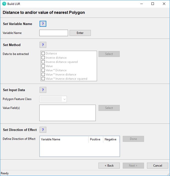
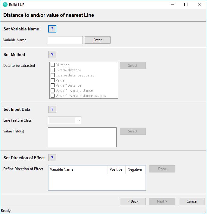
Distance to and/or Value of nearest Polygon

For this type of variable a polygon feature class should be used, which ideally has a spatial extent that is larger than the study area. The polygon feature class must not contain spatial duplicates or invalid geometries (if uncertain about invalid geometries, run the Repair Geometries tool prior to running the wizard).

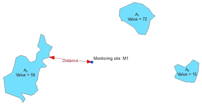
This example diagram shows a feature class of non-contiguous polygons with different values for each feature. For each each point feature representing a monitoring site the wizard will identify the nearest polygon and calculate one or more of the following options:

Distance = The distance to the nearest polygon edge (in the map unit of the projected coordinate system)
Inverse distance = 1 / distance to the nearest polygon edge
Inverse distance squared = 1 / (distance to the nearest polygon edge)²
Value = The value of the nearest polygon
Value * Distance = The value of the nearest polygon x the distance to the nearest polygon edge
Value * Inverse distance = The value of the nearest polygon x (1 / distance to the nearest polygon edge)
Value * Inverse distance squared = The value of the nearest polygon x (1 / (distance to the nearest polygon edge)²)

A real life example of this variable type would be proximity to water bodies with the potential to reduce air temperatures monitored at weather stations or the impact of fugitive emission sources from industrial sites on air quality. Inverse squared distance values are useful to represent the importance of distance, i.e. to give greater importance to nearby polygon features compared with those further away. A Value attribute field might be useful if the size of the feature is important, e.g. livestock densities on agricultural land parcels in the case of ambient ammonia concentrations.

If the monitoring site is located on top of a polygon (i.e. the distance is zero) the Inverse distance, Inverse distance squared, Value * Inverse Distance, and Value * Inverse distance squared options will produce a division by zero error and the result for the feature will be set to missing. The Distance and Value * Distance options will produce a result of zero. Therefore, the user should carefully inspect the data prior to using these options.

Set Variable Name

XLUR Wizard

Set Variable Name

Variable Name

Type in a name for the predictor variable to be created. This must be a unique name, i.e. the same name cannot be assigned to two or more different predictor variables. The name must have a length of at least 1 character and can have a maximum length of 20 characters (ISO basic Latin alphabet). The name cannot contain numbers, spaces or special characters. It is recommended to use a name that will help users to identify the input dataset that the predictor was derived from (e.g. use "forests" rather than "PredictorOne"). Click the Enter button.

Name Schema for Distance to and/or value of nearest Polygon

Predictor variables extracted through this method will appear in the following name schema:

pD_[name entered by user]_[name of value field or none]_[distance method]

where:

pD - set automatically: p indicates that this is a predictor variable, D indicates the type of predictor variable. Click here to see a list of the possible types of predictor variables.
[name entered by user] - set by user: the variable name entered by the user.
[name of value field or none] - set automatically: if only the distance, inverse distance or inverse distance squared is extracted, then this part of the name schema will be set to none. If the methods selected under Set Method include Value, Value * Distance, Value * Inverse distance or Value * Inverse distance squared, then this part of the name schema will be set to the name of the value field selected under Set Input Data.
[distance method] - set automatically:: the distance method used to extract this variable. Distance methods will be set under Set Method and are coded as follows:

Distance method	Code
Distance	dist
Inverse distance	invd
Inverse distance squared	invsq
Value	val
Value * Distance	valdist
Value * Inverse distance	valinvd
Value * Inverse distance squared	valinvsq

Examples:

pD_forest_none_invd - This predictor variable was extracted using a polygon feature class of forests. The naming schema shows that this predictor variable contains the inverse distance to the nearest forest polygon.

pD_forestfire_emission_valinvsq - This predictor variable was extracted using a polygon feature class of forest fires. Each polygon has an emission value and the naming schema shows that this predictor variable contains the inverse squared distance to the nearest forest fire polygon multiplied with the emission value.

Set Method

XLUR Wizard

Set Method

Data to be extracted

Select one or more methods for the data extraction, then click the Select button.

The methods are defined as:

Distance = The distance to the nearest polygon edge (in the map unit of the projected coordinate system)
Inverse distance = 1 ÷ distance to the nearest polygon edge
Inverse distance squared = 1 ÷ (distance to the nearest polygon edge)²
Value = The value of the nearest polygon
Value * Distance = The value of the nearest polygon × the distance to the nearest polygon edge
Value * Inverse distance = The value of the nearest polygon × (1 ÷ distance to the nearest polygon edge)
Value * Inverse distance squared = The value of the nearest polygon × (1 ÷ (distance to the nearest polygon edge)²)

Click here for further details.

Set Input Data

XLUR Wizard

Set Input Data

Polygon Feature Class

From the dropdown menu select the polygon feature class from which you would like to extract data. Ideally, the polygon feature class should have a spatial extent that is larger than the study area. The polygon feature class must not contain spatial duplicates or invalid geometries (if uncertain about invalid geometries, run the Check Geometry or Repair Geometry tool prior to running the wizard). If the Value, Value * Distance, Value * Inverse distance or Value * Inverse distance squared method will be used, the polygon feature class must contain one or more numeric attribute fields.

Value Field(s)

Select one or more fields to be used for the Value, Value * Distance, Value * Inverse distance or Value * Inverse distance squared methods. Please be aware that if the selected value field contains missing data, then the predictor variable will contain missing data, which may cause problems in the statistical analysis.

Set Direction of Effect

XLUR Wizard

Set Direction of Effect

Define Direction of Effect

For example, the distance to a polygon that will increase the dependent variable (i.e. a source polygon) is assumed to have a negative direction of effect (i.e. it is expected to have a negative coefficient), because as distance increases the value of the predictor variable increases, while the actual effect of the polygon decreases. Conversely, the inverse distance and inverse distance squared to a polygon that will increase the dependent variable is assumed to have a positive direction of effect, because as distance increases the calculated value (i.e. 1/distance) of the predictor variable becomes smaller, as does the effect of the polygon.

After all predictor variables in the list have been defined as either positive or negative, click the Done button. A green tick mark will appear and the Next > button will be activated. This completes the Distance to and/or value of nearest Polygon step. The newly created predictor variables will be listed in the Predictors Added box on the next page.

Distance to and/or Value of nearest Line

For this type of variable a line feature class should be used, which ideally has a spatial extent that is larger than the study area. The line feature class must not contain spatial duplicates.

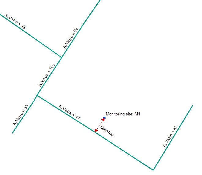
This example diagram shows a line feature class with different values for each feature. For each point feature representing a monitoring site loaction the wizard will identify the nearest line and calculate one or more of the following options:

Distance = The distance to the nearest line (in the map unit of the projected coordinate system)
Inverse distance = 1 / distance to the nearest line
Inverse distance squared = 1 / (distance to the nearest line)² - Value = The value of the nearest line
Value * Distance = The value of the nearest line x the distance to the nearest line
Value * Inverse distance = The value of the nearest line x (1 / distance to the nearest line)
Value * Inverse distance squared = The value of the nearest line x (1 / (distance to the nearest line)²)

A real life example of this variable type would be proximity to the nearest road feature to represent the potential for higher ambient air pollutant concentrations due to vehicular emissions or proximity to the nearest river to represent the potential for lower air temperatures at nearby weather stations. Inverse squared distance values are useful to represent the importance of distance, i.e. to give greater importance to nearby line features compared with those further away. A Value attribute field might be useful if the size of the feature is important, e.g. roads with an attribute representing traffic volume.

If the monitoring site is located on top of a line (i.e. the distance is zero) the Inverse distance, Inverse distance squared, Value * Inverse Distance, and Value * Inverse distance squared options will produce a division by zero error and the result for the feature will be set to missing. The Distance and Value * Distance options will produce a result of zero. Therefore, the user should carefully inspect the data prior to using these options.

Set Variable Name

XLUR Wizard

Set Variable Name

Variable Name

Type in a name for the predictor variable to be created. This must be a unique name, i.e. the same name cannot be assigned to two or more different predictor variables. The name must have a length of at least 1 character and can have a maximum length of 20 characters (ISO basic Latin alphabet). The name cannot contain numbers, spaces or special characters. It is recommended to use a name that will help users to identify the input dataset that the predictor was derived from (e.g. use "RoadsDistance" rather than "PredictorOne"). Click the Enter button.

Name Schema for Distance to and/or value of nearest Line

Predictor variables extracted through this method will appear in the following name schema:

pE_[name entered by user]_[name of value field or none]_[distance method]

where:

pE - set automatically: p indicates that this is a predictor variable, E indicates the type of predictor variable. Click here to see a list of the possible types of predictor variables.
[name entered by user] - set by user: the variable name entered by the user.
[name of value field or none] - set automatically: if only the distance, inverse distance or inverse distance squared is extracted, then this part of the name schema will be set to none. If the methods selected under Set Method include Value, Value * Distance, Value * Inverse distance or Value * Inverse distance squared, then this part of the name schema will be set to the name of the value field selected under Set Input Data.
[distance method] - set automatically:: the distance method used to extract this variable. Distance methods will be set under Set Method and are coded as follows:

Distance method	Code
Distance	dist
Inverse distance	invd
Inverse distance squared	invsq
Value	val
Value * Distance	valdist
Value * Inverse distance	valinvd
Value * Inverse distance squared	valinvsq

Examples:

pE_roads_none_invd - This predictor variable was extracted using a line feature class of roads. The naming schema shows that this predictor variable contains the inverse distance to the nearest road line.

pE_motorwaytraffic_hgv_valinvsq - This predictor variable was extracted using a line feature class of motorways. Each line has an associated count value for heavy goods vehicles (hgv) and the naming schema shows that this predictor variable contains the inverse squared distance to the nearest motorway multiplied by the number of heavy goods vehicles on that motorway.

Set Method

XLUR Wizard

Set Method

Data to be extracted

Select one or more methods for the data extraction, then click the Select button.

The methods are defined as:

Distance = The distance to the nearest line (in the unit of the projected coordinate system)
Inverse distance = 1 ÷ distance to the nearest line
Inverse distance squared = 1 ÷ (distance to the nearest line)²
Value = The value of the nearest line
Value * Distance = The value of the nearest line × the distance to the nearest line
Value * Inverse distance = The value of the nearest line × (1 ÷ distance to the nearest line)
Value * Inverse distance squared = The value of the nearest line × (1 ÷ (distance to the nearest line)²)

Click here for further details.

Set Input Data

XLUR Wizard

Set Input Data

Line Feature Class

From the dropdown menu select the line feature class from which you would like to extract data. Ideally, the line feature class should have a spatial extent that is larger than the study area. The line feature class must not contain spatial duplicates. If the Value, Value * Distance, Value * Inverse distance or Value * Inverse distance squared method will be used, the line feature class must contain one or more numeric fields.

Value Field(s)

Set Direction of Effect

XLUR Wizard

Set Direction of Effect

Define Direction of Effect

For example, the distance to a line that will increase the dependent variable (i.e. a source line) is assumed to have a negative direction of effect (i.e. it is expected to have a negative coefficient), because as distance increases the value of the predictor variable increases, while the actual effect of the line decreases. Conversely, the inverse distance and inverse distance squared to a line that will increase the dependent variable is assumed to have a positive direction of effect, because as distance increases the calculated value (i.e. 1/distance) of the predictor variable becomes smaller, as does the effect of the line.

After all predictor variables in the list have been defined as either positive or negative, click the Done button. A green tick mark will appear and the Next > button will be activated. This completes the Distance to and/or value of nearest Line step. The newly created predictor variables will be listed in the Predictors Added box on the next page.

Distance to and/or Value of nearest Point

For this type of variable a point feature class should be used, which ideally has a spatial extent that is larger than the study area. The point feature class must not contain spatial duplicates.

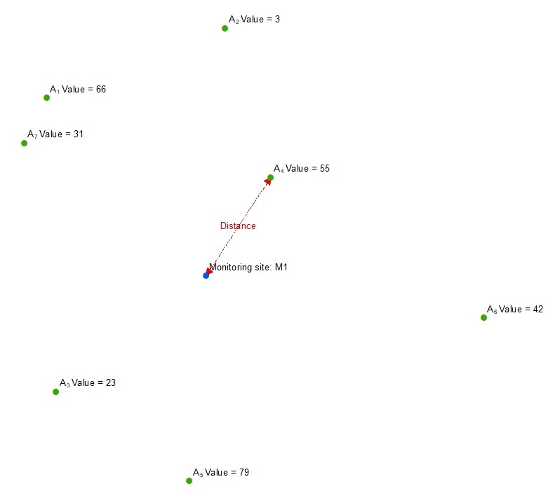
This example diagram shows a point feature class with different values for each feature. For each monitoring site the wizard will identify the nearest point and calculate one or more of the following options:

Distance = The distance to the nearest point (in the map unit of the projected coordinate system)
Inverse distance = 1 / distance to the nearest point
Inverse distance squared = 1 / (distance to the nearest point)² - Value = The value of the nearest point
Value * Distance = The value of the nearest point x the distance to the nearest point
Value * Inverse distance = The value of the nearest point x (1 / distance to the nearest point)
Value * Inverse distance squared = The value of the nearest point x (1 / (distance to the nearest point)²)

A real life example of this variable type would be proximity to the nearest point feature representing a chimney stack. In this case closer distances are more likely to result in higher pollutant concentrations. Inverse squared distance values are useful to represent the importance of distance, i.e. to give greater importance to nearby point features compared with those further away. A Value attribute field might be useful if the size of the feature is important, e.g. the emission rate from the chimney stack.

If the monitoring site is located on top of a point (i.e. the distance is zero) the Inverse distance, Inverse distance squared, Value * Inverse Distance, and Value * Inverse distance squared options will produce a division by zero error and the result for the feature will be set to missing. The Distance and Value * Distance options will produce a result of zero. Therefore, the user should carefully inspect the data prior to using these options.

Set Variable Name

XLUR Wizard

Set Variable Name

Variable Name

Type in a name for the predictor variable to be created. This must be a unique name, i.e. the same name cannot be assigned to two or more different predictor variables. The name must have a length of at least 1 character and can have a maximum length of 20 characters (ISO basic Latin alphabet). The name cannot contain numbers, spaces or special characters. It is recommended to use a name that will help users to identify the input dataset that the predictor was derived from (e.g. use "ChimneyDist" rather than "PredictorOne"). Click the Enter button.

Name Schema for Distance to and/or value of nearest Point

Predictor variables extracted through this method will appear in the following name schema:

pF_[name entered by user]_[name of value field or none]_[distance method]

where:

pF - set automatically: p indicates that this is a predictor variable, F indicates the type of predictor variable. Click here to see a list of the possible types of predictor variables.
[name entered by user] - set by user: the variable name entered by the user.
[name of value field or none] - set automatically: if only the distance, inverse distance or inverse distance squared is extracted, then this part of the name schema will be set to none. If the methods selected under Set Method include Value, Value * Distance, Value * Inverse distance or Value * Inverse distance squared, then this part of the name schema will be set to the name of the value field selected under Set Input Data.
[distance method] - set automatically: the distance method used to extract this variable. Distance methods will be set under Set Method and are coded as follows:

Distance method	Code
Distance	dist
Inverse distance	invd
Inverse distance squared	invsq
Value	val
Value * Distance	valdist
Value * Inverse distance	valinvd
Value * Inverse distance squared	valinvsq

Examples:

pF_chimneystack_none_invd - This predictor variable was extracted using a point feature class of chimney stacks. The naming schema shows that this predictor variable contains the inverse distance to the nearest chimney stack.

pF_altitude_height_val - This predictor variable was extracted using a point feature class of altitudes. Each point has an associated height above sea level value and the naming schema shows that this predictor variable contains the height above sea level of the nearest point.

Set Method

XLUR Wizard

Set Method

Data to be extracted

Select one or more methods for the data extraction, then click the Select button.

The methods are defined as:

Distance = The distance to the nearest point (in the unit of the projected coordinate system)
Inverse distance = 1 ÷ distance to the nearest point
Inverse distance squared = 1 ÷ (distance to the nearest point)²
Value = The value of the nearest point
Value * Distance = The value of the nearest point × the distance to the nearest point
Value * Inverse distance = The value of the nearest point × (1 ÷ distance to the nearest point)
Value * Inverse distance squared = The value of the nearest point × (1 ÷ (distance to the nearest point)²)

Click here for further details.

Set Input Data

XLUR Wizard

Set Input Data

Point Feature Class

From the dropdown menu select the point feature class from which you would like to extract data. Ideally, the point feature class should have a spatial extent that is larger than the study area. The point feature class must not contain spatial duplicates. If the Value, Value * Distance, Value * Inverse distance or Value * Inverse distance squared method will be used, the point feature class must contain one or more numeric fields.

Value Field(s)

Set Direction of Effect

XLUR Wizard

Set Direction of Effect

Define Direction of Effect

For example, the distance to a point that will increase the dependent variable (i.e. a source point) is assumed to have a negative direction of effect (i.e. it is expected to have a negative coefficient), because as distance increases the value of the predictor variable increases, while the actual effect of the point decreases. Conversely, the inverse distance and inverse distance squared to a point that will increase the dependent variable is assumed to have a positive direction of effect, because as distance increases the calculated value (i.e. 1/distance) of the predictor variable becomes smaller, as does the effect of the point.

After all predictor variables in the list have been defined as either positive or negative, click the Done button. A green tick mark will appear and the Next > button will be activated. This completes the Distance to and/or value of nearest Point step. The newly created predictor variables will be listed in the Predictors Added box on the next page.

Raster based Predictors

Value of Raster cell

You must have a Spatial Analyst license to create this type of predictor. For this type of variable a raster grid file should be used, which ideally has a spatial extent that is larger than the study area. The wizard will extract the value of the raster cell that is spatially coincident with the point location representing the monitoring site (dependent variable).

An example of the use of this predictor variable type is elevation. Elevation is commonly sourced from a Digital Elevation Model stored as a raster grid.

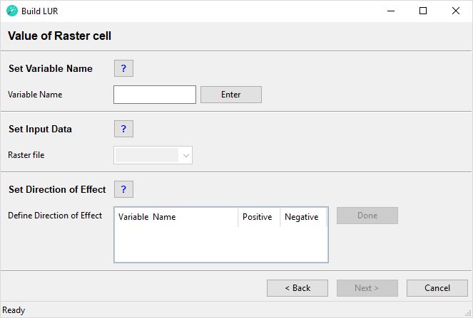
Set Variable Name

XLUR Wizard

Set Variable Name

Variable Name

Type in a name for the predictor variable to be created. This must be a unique name, i.e. the same name cannot be assigned to two or more different predictor variables. The name must have a length of at least 1 character and can have a maximum length of 20 characters (ISO basic Latin alphabet). The name cannot contain numbers, spaces or special characters. It is recommended to use a name that will help users to identify the input dataset that the predictor was derived from (e.g. use "altitude" rather than "PredictorOne"). Click the Enter button.

Name Schema for Value of nearest Raster cell

Predictor variables extracted through this method will appear in the following name schema:

pG_[name entered by user]_raster_val

where:

pG - set automatically: p indicates that this is a predictor variable, G indicates the type of predictor variable. Click here to see a list of the possible types of predictor variables.
[name entered by user] - set by user: the variable name entered by the user.
raster_val - set automatically: shows that this is a value extracted from a raster file.

Example:

pG_digiterrain_raster_val - This predictor variable was extracted from a raster file of digital terrain data. The naming schema shows that a cell value from a raster file was extracted.

Set Input Data

XLUR Wizard

Set Input Data

Raster file

From the dropdown menu select the raster grid file from which you would like to extract data. Since raster files cannot be imported into feature datasets directly, a raster file called pG_[name entered by user] will be created in the input file geodatabase.

Set Direction of Effect

XLUR Wizard

Set Direction of Effect

Define Direction of Effect

Select whether the predictor variable is expected to have a positive or a negative direction of effect. The user has to make an a priori assumption for each predictor variable: a positive direction of effect is a predictor variable that will increase the value of the dependent variable, i.e. it is considered to be a source of the dependent variable and the beta coefficient is expected to be positive. A negative direction of effect is a predictor variable that will decrease the value of the dependent variable, i.e. it is considered to be a sink of the dependent variable and the beta coefficient is expected to be negative. These specifications will be used as model selection criteria in the statistical analysis; therefore, the user must consider carefully whether each predictor variable has a positive or a negative direction of effect. Incorrect specifications will lead to incorrect LUR models!

Click the Done button. A green tick mark will appear and the Next > button will be activated. This completes the Value of Raster cell step. The newly created predictor variables will be listed in the Predictors Added box on the next page.

Step 4 - Model

This is the final step of the Build LUR wizard. In this step the LUR model will be created.

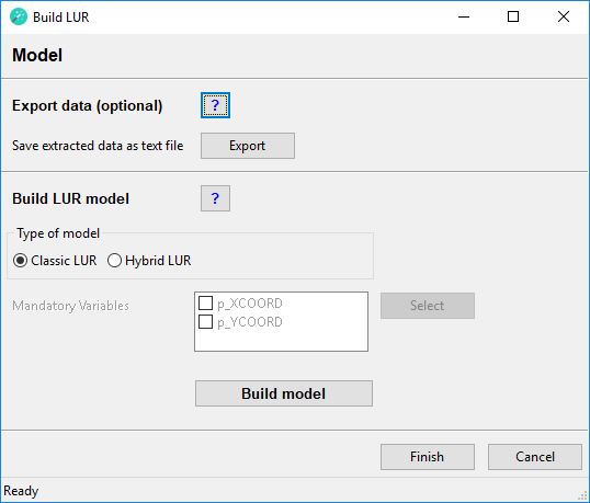
Export data

XLUR Wizard

Export data (optional)

Save extracted data as text file

Click the Export button to save a comma separated text file of the dependent and predictor variables. The file will be saved in the output folder. This file is useful, if the user wishes to run statistical analyses independent of the wizard.

Build LUR Model

XLUR Wizard

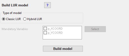
Build LUR model

Type of model

Select the type of model you wish to run. The Classic LUR uses the variable selection strategy established in the ESCAPE study (Click here to open the ESCAPE Exposure assessment manual). The Hybrid LUR will enter one or more mandatory variables into the regression model prior to starting the variable selection procedure following the methodology described in de Hoogh et al.(2016) DOI: 10.1016/j.envres.2016.07.005.

Mandatory Variables

Select one or more mandatory variables to be entered into the hybrid LUR model. Then click the Select button. A green tick mark will appear and the Build model button will be enabled.

Build model

Click this button to build the LUR model. Once the model has been built a green tick mark will appear. Click the Finish button to close the wizard tool. The log file saved in the output folder contains details of the LUR models that have been created. The coefficients of the LUR models have also been stored in the SQLite database, to be used in the Apply LUR model tool. Descriptive statistics, model diagnostic plots and residuals have also been saved in the output folder. These allow consideration of the reliability of the models and checking of possible input errors (e.g. incorrect specification of the direction of effect).

Apply LUR

To apply a LUR model built with the wizard to estimate values for a number of receptor point locations double-click the ApplyLUR script in the XLUR toolbox. The ApplyLUR tool will appear in the Geoprocessing pane. Click the Run button in the bottom right corner to run the tool.

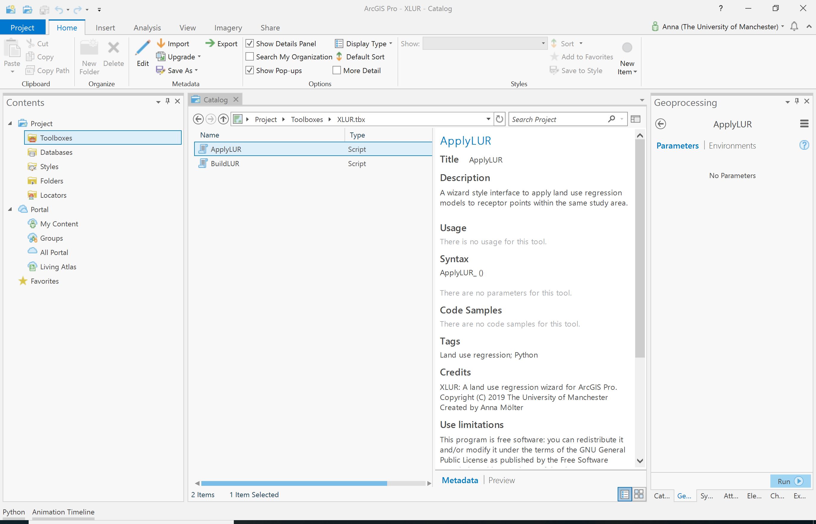
This will open the ApplyLUR wizard. The wizard will guide you through the process of applying a LUR model by using the following steps:

Step 1 - Settings

This step is required to specify some general settings to apply a LUR model.

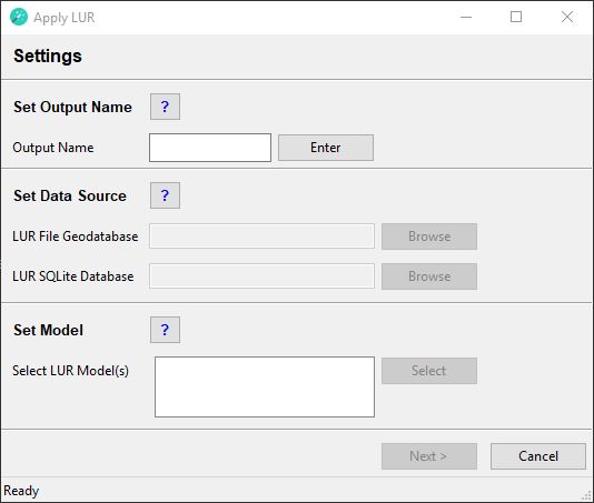
Set Output Name

XLUR Wizard

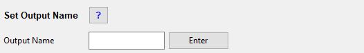
Set Output Name

Output Name

Type in a name to identify your LUR output files. The name must have a length of a at least 1 character and can have a maximum length of 10 characters. The name can contain text (ISO basic Latin alphabet), numbers and underscores. The name must start with a text character.

The name will be used to create a new folder in your Build LUR output folder. The new folder will use the following name schema: [name entered by user]_[current Date]_[current Time]. Inside this new folder a new File Geodatabase, a new SQLite Database, a new Error File and a new Log file will be created. These will contain all the data relevant to the outputs for the receptor points. Modelled values for the receptor point locations will be stored in a feature class called [name entered by user]_receptors in the File Geodatabase.

Click the Enter button to continue.

Set Data Source

XLUR Wizard

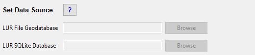
Set Data Source

LUR File Geodatabase

Click on the Browse button to open the directory dialog. Navigate to the output folder that was created during the Build LUR step. In this folder select the File Geodatabase containing the LUR data. This must be a folder with a '.gdb' extension. Click the Select Folder button. The file path to the LUR File Geodatabase and a green tick mark will appear. Depending on the size of the File Geodatabase this may take a while.

LUR SQLite Database

Click on the Browse button to open the directory dialog. Navigate to the output folder that was created during the Build LUR step. In this folder select the LurSqlDB.sqlite file. Click the Select Folder button. The file path to the LUR SQLite Database and a green tick mark will appear.The LUR models stored in the SQLite database will be listed in the Set Model section.

Set Model

XLUR Wizard

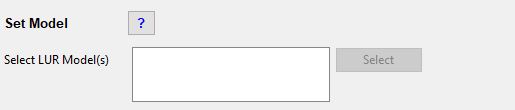
Set Model

Select LUR Model(s)

Select one or more LUR models that you wish to use. The Build LUR tool can develop multiple models simultaneously, depending on the number of dependent variables selected in Step 2 - Outcomes. This means multiple LUR models may be available in this box and these can be applied simultaneously. Please be aware that the processing time of the tool will increase, if multiple models are selected. The name of the model indicates which outcome will be modelled. Click the Select button. A green tick mark will appear and the Next > button will be activated. After the Next > has been clicked, it may take some time to display the next page. This is because source data is being copied from the LUR File Geodatabase into the output File Geodatabase.

This completes the Settings step.

Step 2 - Receptors

This step is required to specify the receptor locations. Receptor locations must be point feature classes. They denote the locations for which estimates of the value of the dependent variable will be made.

XLUR Wizard

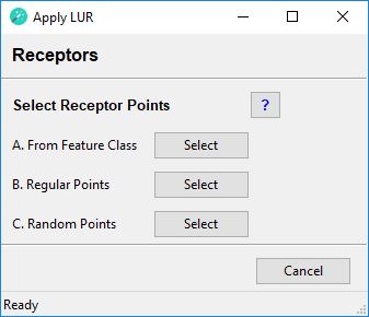
Select Receptor Points

Receptor points to be used by the Apply LUR wizard can be derived from three sources:

A. From Feature Class

The user must specify a point feature class that contains the receptor points.

B. Regular Points

A set of points at specified regular intervals is created across the study area.

C. Random Points

A number (n) of random points are created within the study area, where n is specified by the user.

From Feature Class

XLUR Wizard

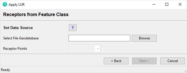
Set Data Source

Select File Geodatabase

Click on the Browse button to open the directory dialogue. Navigate to the File Geodatabase that contains your receptor points. This must be a folder with a '.gdb' extension. Click the Select Folder button. The file path to the File Geodatabase and a green tick mark will appear. The dropdown menu below will be populated with the names of all point feature classes in this File Geodatabase. Depending on the size of the File Geodatabase this may take a while.

Receptor Points

From the dropdown menu, select the feature class that contains the receptor points. It is recommended to use a feature class that does not contain spatial duplicates, as the presence of spatial duplicates will slow down the performance of the tool.

A green tick mark will appear and the Next > button will be activated. This completes the Receptors from Feature Class step.

If the LUR models contain predictors that are derived from the Inverse distance, Inverse distance squared, Value * Inverse Distance, or Value * Inverse distance squared to the nearest feature, then any receptor points located on top of the nearest feature will result in a division by zero error, because the distance is zero. To prevent this, the wizard will check if the LUR model contains an Inverse distance, Inverse distance squared, Value * Inverse Distance, or Value * Inverse distance squared predictor. If this is the case, the wizard will remove any receptor points located on top of the relevant features. The warning message "Invalid receptor points. See log for details." will appear and the Apply_LOG will record which predictor variable resulted in the removal of receptor points. The Apply_LOG will also record the initial and final number of receptor points used.

Regular Points

XLUR Wizard

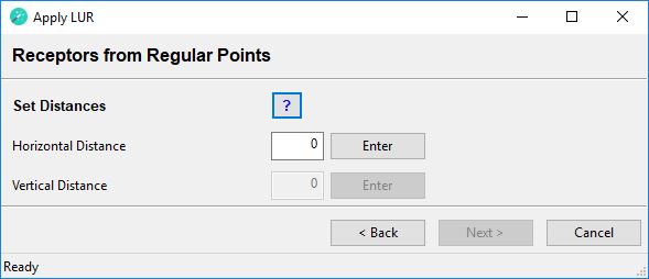
Set Distances

Horizontal Distance

Type in the required distance between grid points in the horizontal direction, i.e. along the X axis (East-West). The unit of the distance is the same as the map unit of the projected coordinate system of your study area. Click the Enter button. A green tick mark will appear and the Vertical Distance input field will be activated.

Vertical Distance

Type in the required distance between grid points in the vertical direction, i.e. along the Y axis (North-South). The unit of the distance is the same as the map unit of the projected coordinate system of your study area. Click the Enter button. A green tick mark will appear and the Next > button will be activated. This completes the Receptors from Regular Points step.

Random Points

XLUR Wizard

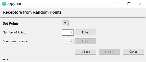
Set Points

Number of Points

Type in the number of random points that you would like to create within the study area. Click the Enter button. A green tick mark will appear and the Minimum Distance input field will be activated.

Minimum Distance

Type in the minimum distance that receptor points should be apart. This must be a number greater than zero. The unit of the distance is the same as the map unit of the projected coordinate system of your study area. It is recommended to use a minimum distance equal to or greater than 2x the smallest buffer size used in the LUR model. Click the Enter button. A green tick mark will appear and the Next > button will be activated. This completes the Receptors from Random Points step.

Step 3 - Apply Model

This is the final step, which will apply the LUR model to the receptor points.

XLUR Wizard

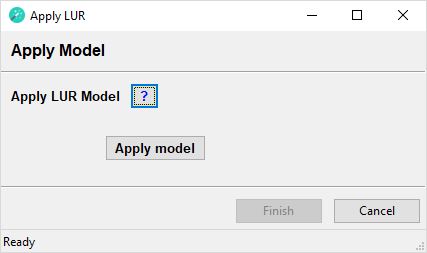
Apply LUR model

Apply model

Click this button to apply the LUR model(s) to the receptor points. Applying the LUR model(s) may take a while depending on the number of models, complexity of the models and data, and number of receptor points. If the apply stage seems excessively long, look at the messages at the bottom of the Geoprocessing pane (hover over ApplyLUR or toggle the Show or Hide Messages button to see messages). If you see the following message "+++ERROR+++ Uncaught exception -> See GOTCHA" an error has occured. Open the GOTCHA file for more information.

Once the model has been applied a green tick mark will appear. Modelled values will be stored in the pred_lyr feature class in the File Geodatabase. Click the Finish button to close the wizard tool.

Troubleshooting

Known issues

After closing the XLUR project and exiting ArcGIS Pro you may see a warning message similar to this one:

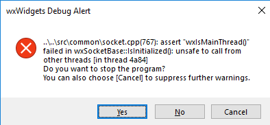
This is a warning only, it is not a critical error. This is a known issue and it has been reported to ESRI as a potential bug.

Running the XLUR tools repeatedly may cause ArcGIS Pro to crash. This may be related to the warning shown in issue 1. It is recommended to restart ArcGIS Pro between separate runs of the XLUR tools.

Frequently Asked Questions

In my data each land use type is stored in an individual feature class. How can I use these data?

Add a text field to each feature class. In each feature class set all rows of this new text field to the same value. For example, you could set all rows to show the name of the type of land use that is stored in this feature class.

I cannot read the full name of an option in a dropdown menu, because the name is very long

Enlarge the window by dragging its right side or click the maximise button in the title bar.

I cannot see the Finish button on the Model page

Enlarge the window by clicking the maximise button in the title bar.

Some of my receptor points were not modelled by the ApplyLUR tool

Please inspect your receptor points carefully on a map and look at the predictor variables in your LUR models. If the LUR models contain predictors that are derived from the Inverse distance, Inverse distance squared, Value * Inverse Distance, or Value * Inverse distance squared to the nearest feature method, then any receptor points spatially coincident with the nearest feature will be dropped to prevent a division by zero error.

The Build LUR tool freezes when I use the Value of Raster cell page

Please check that you have a license for Spatial Analyst.

Tutorial

This section provides a guided tutorial for building and applying a LUR model using the XLUR wizard. In this tutorial you will build and apply a predictive air pollution model for the Greater Manchester area using openly accessible datasets on monitored Nitrogen Dioxide (NO₂) concentrations, land use categories, road networks, and emission sources. Please note that the purpose of this tutorial is to illustrate the use of the XLUR wizard, not to develop a high performing LUR model; therefore, only a small number of input datasets are used in this tutorial.

Before you start

Ensure that you have cloned or downloaded the XLUR repository from GitHub, including the ExampleData folder.
Follow the instructions in the Installation section to ensure that the additional Python packages required by XLUR have been installed and that you have a license for Spatial Analyst.
Create a directory where you would like to store outputs from the model, for example C:\Work\XLUROutput. Please ensure that you have write access to this directory and that there are no spaces in the file path.

Starting the XLUR wizard

Start ArcGIS Pro and open the XLUR project. The XLUR.aprx project file can be found in the XLUR folder in the XLUR repository.
In the Catalog window right-click Folders and click Add Folder Connection. Create a connection to the ExampleData.gdb file geodatabase, which is stored in the ExampleData folder in the XLUR repository.
Double-click toolboxes, double-click XLUR.tbx, then double-click the BuildLUR script. In the Geoprocessing window on the right click Run. This will open the Build LUR wizard.

If at any time you require more information on a specific section, click on the question mark button next to the section heading. This will open a help window with further information on how to complete each section.

Settings

On this page you will specify the general settings required by XLUR wizard.

Set Project Name
- Next to Project Name type a suitable name for your LUR model (e.g. MyFirstLUR) and click Enter.
Set Directories
- Click the Browse button next to Input File Geodatabase and navigate to ExampleData.gdb.
- Click the Browse button next to Output Folder and navigate to the directory where you would like to store outputs from the model.
Set Coordinate System
- You must specify a projected coordinate system for the data. The help menu provides a link to the well-known ID (WKID) numbers for the coordinate systems provided in ArcGIS Pro. In this tutorial you will use the British National Grid projected coordinate system. Its WKID is 27700.
Set Study Area
- From the dropdown menu select GMArea.

The completed Settings page should look like this:

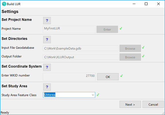
Click Next > to continue.

Outcomes

On this page you will specify the data that will be used as the outcome that the LUR model needs to predict. In this tutorial the outcome is annual average Nitrogen Dioxide concentrations measured by diffusion tubes in the Greater Manchester area.

Set Dependent Variable
- From the dropdown menu next to Monitoring Sites select GMDiffusionTubes.
- From the dropdown menu next to Select Site ID select SiteID.
- In the box next to Dependent Variables tick NO2, then click Select. In the box below Outcomes Added depNO2 should appear.

The completed Outcomes page should look like this:

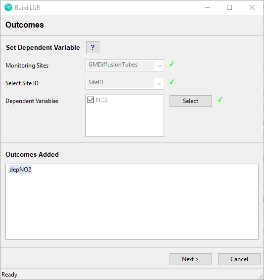
Click Next > to continue.

Predictors

On the next pages you will specify potential predictors for the LUR model. Potential predictor variables fall into seven types and further information on these types is provided in the help menu. You can add as many or as few predictors as you wish. You can see in the box below Predictors Added that the coordinates of each monitoring site have been automatically added as potential predictor variables.

Click the Add button next to A. Polygon Area or Value within Buffer.

Polygon Area or Value within Buffer

Through this page you will create potential predictor variables that are based on drawing circular buffers around each monitoring site and extracting the area or attribute value from a polygon feature class that intersects these buffers. For the purpose of this tutorial you will create predictors that show the area of different land use categories within each buffer.

Set Variable Name
- In the box next to Variable Name type a name for the variable to be created, e.g. landuseArea, then click Enter.
Set Buffer Sizes
- Under Buffers select Create new buffer.
- In the box next to Create Buffer Distance type in 100 (this will create a buffer with a radius of 100m), then click Add. The buffer distance that you have added will appear in the box below.
- Repeat this step to add buffer distances of 300, 500, 1000, and 5000. If you make a mistake, select the incorrect buffer distance and click remove.
- Once all buffer distances have been entered click Done.
Set Input Data
- From the dropdown menu next to Polygon Feature Class select CorineLanduse.
- From the dropdown menu next to Category Field select LanduseCat.
- Under Aggregation Method select Total area.
Set Direction of Effect
- The box next to Define Direction of Effect is automatically populated with the names of the predictor variables that will be created. In this case the variable name includes the name that was entered at the top of the page (landuseArea), the names of the land use categories (HDres,Industry,LDres,Natural,UrbGreen,Port), the buffer distances (100,300,500,1000,5000), and the aggregation method (sum indicates that the total area within the buffer will be used). For each predictor variable you must now select whether the a priori assumed direction of effect of the predictor is positive or negative. This is a critical step, for further information on this click the help button. In an air pollution study it is usually assumed that urban and industrial land uses increase pollution levels, i.e. their direction of effect will be positive, while natural land uses decrease pollution levels, i.e. their direction of effect will be negative. Scroll through the list of predictor variables and set all HDres, Industry, LDres, and Port variables to Positive. Set all Natural and UrbGreen variables to Negative, then click done.

The completed page should look like this:

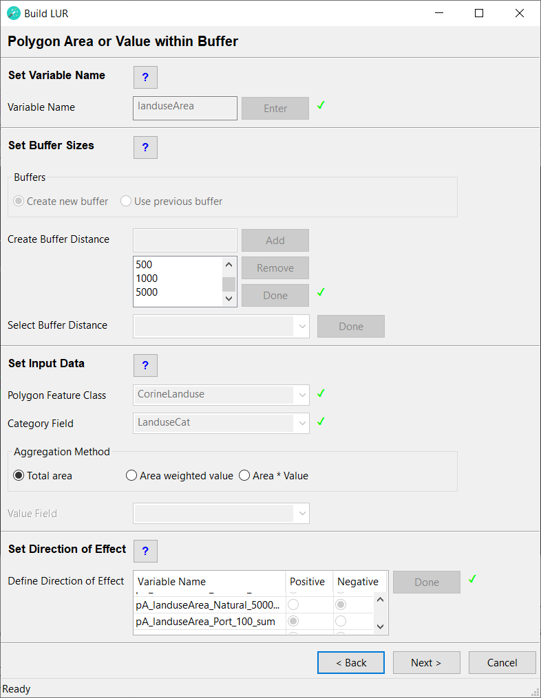
Click Next > to continue. The Predictors page will open again (this may take a while). You can see that in the box below Predictors Added the new predictors have been added together with their assumed direction of effect.

You will now create predictors that show oxides of nitrogen (NOx) emitted from the area within buffers surrounding the monitoring sites. Data on NOx emission rates comes in different formats and for this predictor variable you will use emission rates aggregated at an area level (in this case regular square polygons). Since the buffers do not match the emission polygons exactly, the emission rate values need to be area weighted.

Click the Add button next to A. Polygon Area or Value within Buffer.

Set Variable Name
- In the box next to Variable Name type a name for the variable to be created, e.g. EmissionAreaWt, then click Enter.
Set Buffer Sizes
- Under Buffers select Use previous buffer.
- From the dropdown menu next to Select Buffer Distance select [100, 300, 500, 1000, 5000]. Make sure to click on this set of distances, to select it (it will briefly appear with a blue background, if it has been selected).
- Click Done.
Set Input Data
- From the dropdown menu next to Polygon Feature Class select TotalNoxEmissionAsNO2_Tiles.
- From the dropdown menu next to Category Field select DummyCat. Since categories are not relevant for this dataset a dummy variable has been added, which assigns all polygons to the same category.
- Under Aggregation Method select Area weighted value.
- From the dropdown menu next to Value Field select NOxEmission.
Set Direction of Effect
- The box next to Define Direction of Effect shows the names of the predictor variables that will be created. For these variables the name includes the name that was entered at the top of the page (EmissionAreaWt), the name in the dummy category (All), the buffer distances (100,300,500,1000,5000), and the aggregation method (wtv indicates that an area weighted value will be used). This type of predictor variable represents emission rates of pollution, therefore its direction of effect is obviously assumed to be positive. Scroll through the list of predictor variables and set all variables to Positive, then click done.

The completed page should look like this:

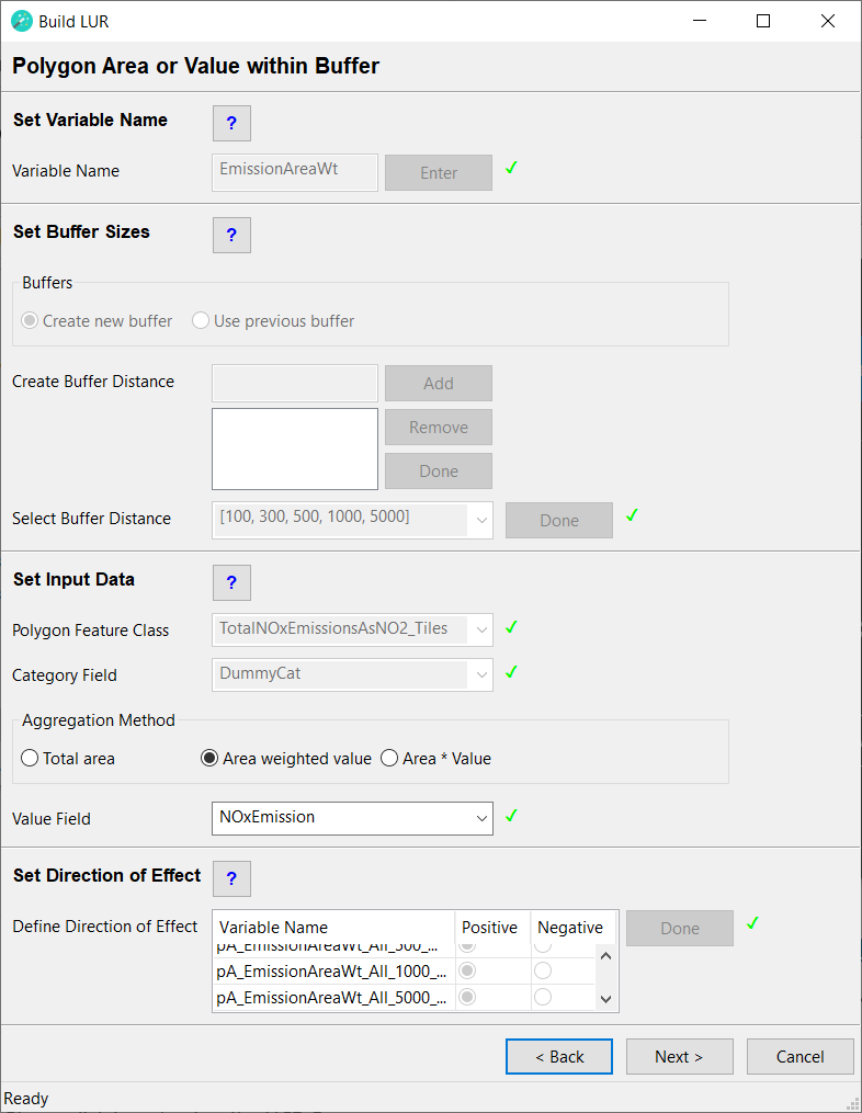
Click Next > to continue. You may see a Warning box. Click OK and the warning will disappear and the Predictors page will open (this may take a while).

Click the Add button next to B. Line Length or Value within Buffer.

Line Length or Value within Buffer

Through this page you will create potential predictor variables that are based on drawing circular buffers around each monitoring site and extracting the length or attribute value from a line feature class that intersects these buffers. For this tutorial you will create predictors that show the lengths of major and minor roads within each buffer.

Set Variable Name
- In the box next to Variable Name type a name for the variable to be created, e.g. rdLength, then click Enter.
Set Buffer Sizes
- Under Buffers select Create new buffer.
- For the buffer distances enter 25, 50, 100, 300, 500, and 1000.
Set Input Data
- From the dropdown menu next to Line Feature Class select OSM_AllRoads.
- From the dropdown menu next to Category Field select RoadCat.
- Under Aggregation Method select Total length.
Set Direction of Effect
- Traffic is a major source of air pollution in urban areas. Therefore, it is expected that a higher road density will increase pollution levels. Scroll through the list of predictor variables and set all variables to Positive, then click Done

The completed page should look like this:

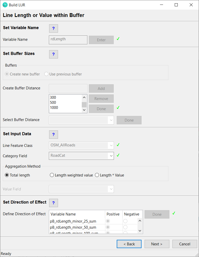
Click Next > to continue. The Predictors page will open again (this may take a while).

Click the Add button next to C. Point Count or Value within Buffer.

Point Count or Value within Buffer

Through this page you will create potential predictor variables that are based on drawing circular buffers around each monitoring site and extracting the number of points or a statistic of their attribute values from a point feature class that intersects these buffers. In this case you will create predictors that show the sum of NOx emissions from point sources within each buffer by industry sector.

Set Variable Name
- In the box next to Variable Name type a name for the variable to be created, e.g. EmissionPoint, then click Enter.
Set Buffer Sizes
- Under Buffers select Use previous buffer.
- From the dropdown menu next to Select Buffer Distance select [100, 300, 500, 1000, 5000]. Make sure to click on this set of distances, to select it (it will briefly appear with a blue background, if it has been selected).
- Click Done.
Set Input Data
- From the dropdown menu next to Point Feature Class select NOxEmissionPointSources.
- From the dropdown menu next to Category Field select SectorCat.
- Under Aggregation Method select Sum of values.
- From the dropdown menu next to Value Field select Emission.
Set Direction of Effect
- Since emission sources will increase pollution levels, the direction of effect of all variables should be set to Positive. Click Done.

The completed page should look like this:

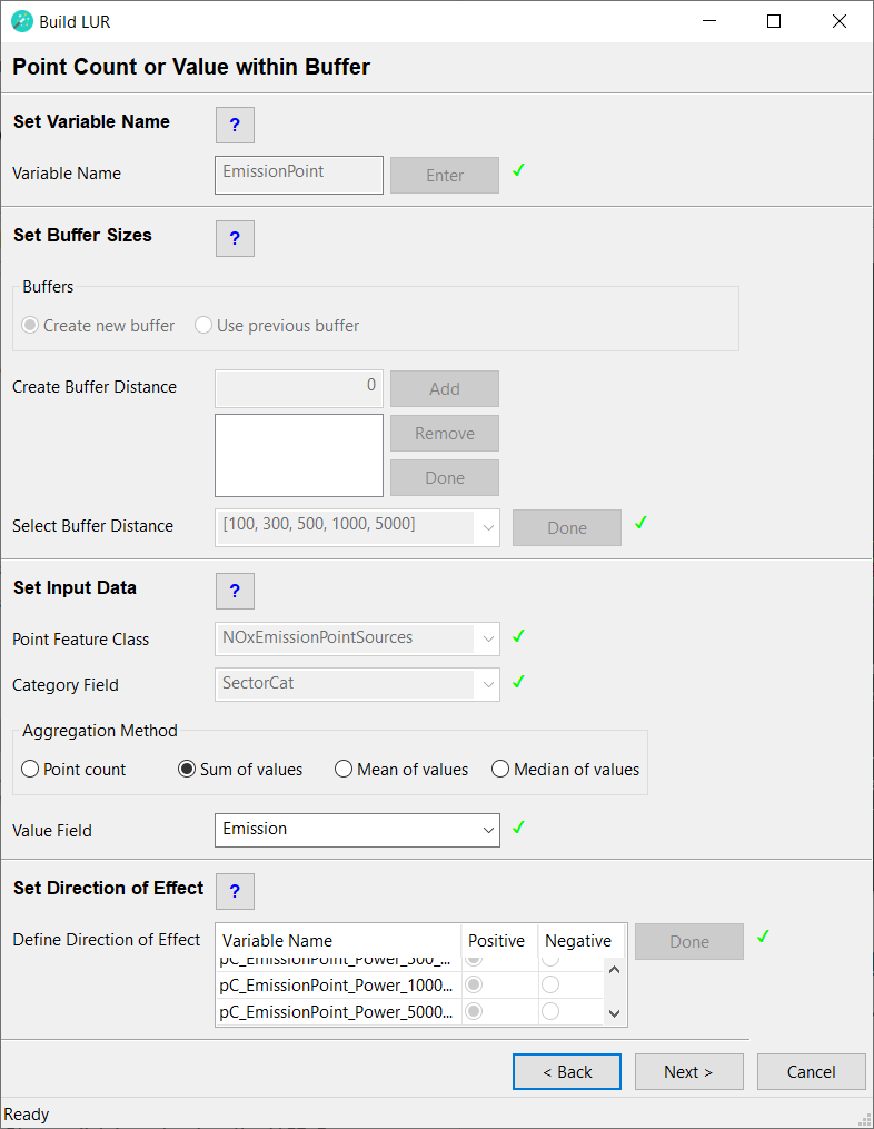
Click Next > to continue. The Predictors page will open again (this may take a while).

Click the Add button next to D. Distance to and/or Value of nearest Polygon.

Distance to and/or value of nearest Polygon

Through this page you will create potential predictor variables that show the distance from each monitoring site to the nearest polygon, or the value of the nearest polygon or a combination of the distance and the value. As shown above NOx emission sources can be processed in different formats: as point sources or aggregated to an area level (as square polygons). For the purpose of this tutorial you will extract an area level emission rate for each monitoring site, which will be the emission rate of the polygon that the monitoring site is located on.

Set Variable Name
- In the box next to Variable Name type a name for the variable to be created, e.g. EmissionAreaVal, then click Enter.
Set Method
- In the box next to Data to be extracted tick Value, then click Select.
Set Input Data
- From the dropdown menu next to Polygon Feature Class select TotalNoxEmissionAsNO2_Tiles.
- In the box next to Value Field(s) tick NOxEmission, then click Select.
Set Direction of Effect
- Again, as NOx emissions increase, air pollution levels will increase; therefore, the direction of effect should be set to Positive. Click Done.

The completed page should look like this:

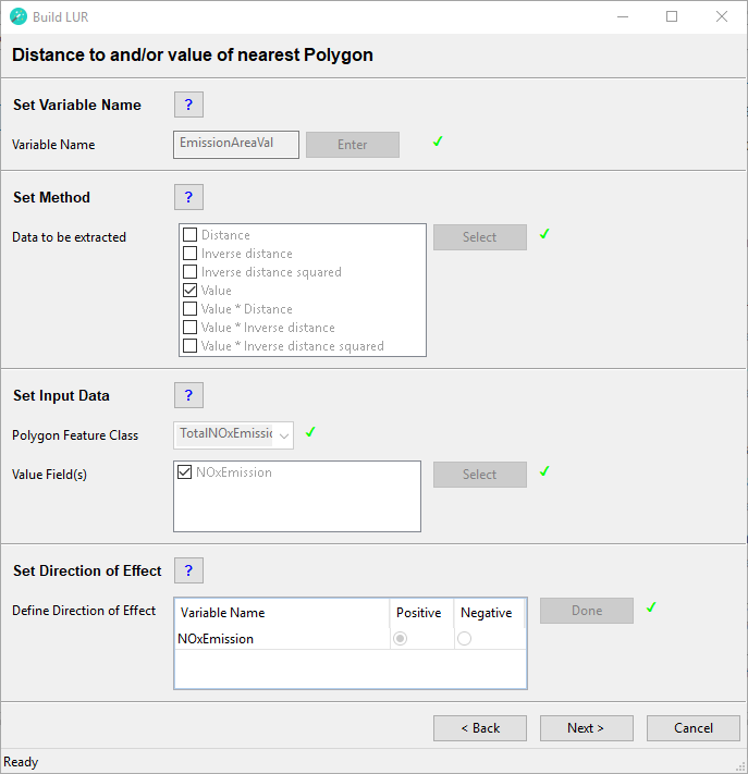
Click Next > to continue. The Predictors page will open again.

Click the Add button next to E. Distance to and/or Value of nearest Line.

Distance to and/or value of nearest Line

Through this page you will create potential predictor variables that show the distance from each monitoring site to the nearest line, or the value of the nearest line or a combination of the distance and the value. For this tutorial you will extract the distance, inverse distance and inverse distance squared from each monitoring site to the nearest major road.

Set Variable Name
- In the box next to Variable Name type a name for the variable to be created, e.g. majorRdDist, then click Enter.
Set Method
- In the box next to Data to be extracted tick Distance, Inverse distance and Inverse distance squared, then click Select.
Set Input Data
- From the dropdown menu next to Line Feature Class select OSM_MajorRoads.
Set Direction of Effect
- The further away a monitoring site is from a road the less it will be influenced by emissions from traffic on the road. This means as distance increases, pollution levels will decrease; therefore, you should set the direction of effect of the Distance variable to Negative. The inverse distance is 1 divided by the distance, while the inverse distance squared is 1 divided by the squared distance. This means as the distance becomes larger the inverse distance and inverse distance squared become smaller and so do the pollution levels. Therefore, you should set the direction for the Inverse distance and Inverse distance squared variables to Positive, then click Done. It is usually not necessary to use both the Distance and the Inverse distance, as they are functions of each other. However, for the purpose of this tutorial both are included to illustrate the fact that they have opposite directions of effects.

The completed page should look like this:

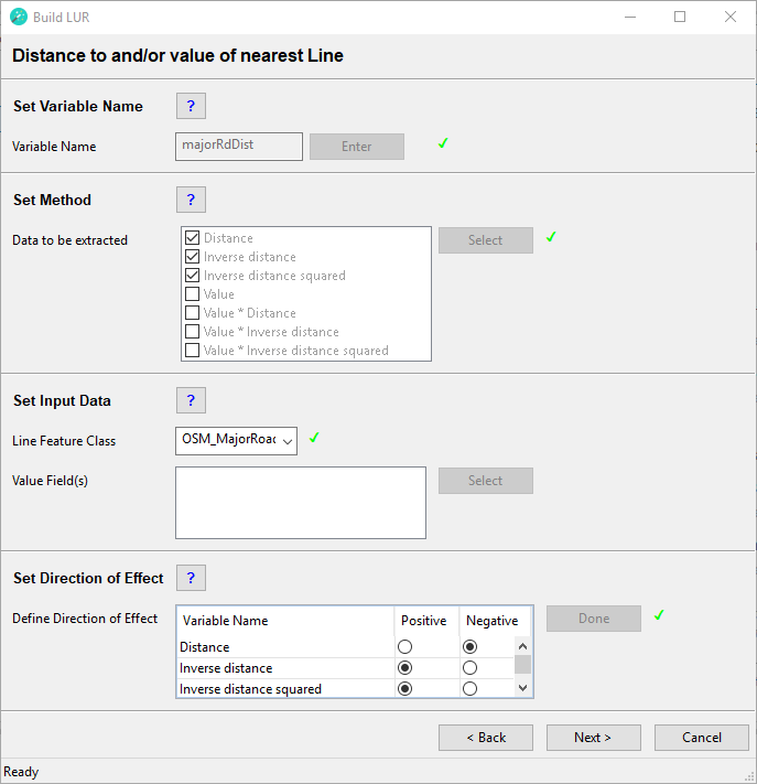
Click Next > to continue. The Predictors page will open again.

Click the Add button next to F. Distance to and/or Value of nearest Point.

Distance to and/or value of nearest Point

Through this page you will create potential predictor variables that show the distance from each monitoring site to the nearest point, or the value of the nearest point or a combination of the distance and the value. For this tutorial you will extract the emission rate*inverse distance and the emission rate*inverse distance squared from each monitoring site to the nearest point source of NOx.

Set Variable Name
- In the box next to Variable Name type a name for the variable to be created, e.g. EmPoint, then click Enter.
Set Method
- In the box next to Data to be extracted tick Value * Inverse distance and Value * Inverse distance squared, then click Select.
Set Input Data
- From the dropdown menu next to Point Feature Class select NOxEmissionPointSources.
- In the box next to Value Field(s) tick Emission, then click Select.
Set Direction of Effect
- As illustrated above when using the inverse distance and inverse distance squared the value of the predictor variable changes in the same direction as does the pollution levels; therefore, the direction of effect for both variables should be set to Positive. Click Done.

The completed page should look like this:

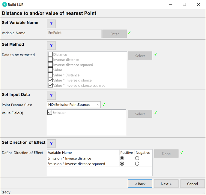
Click Next > to continue. The Predictors page will open again.

If you have a Spatial Analyst license, click the Add button next to G. Value of Raster cell. If you do not have a Spatial Analyst license, skip this step and click Next >.

Value of Raster cell

Through this page you will create potential predictor variables that show the value of the raster cell that each monitoring site location spatially coincident with. For this you will use NOx emission rates aggregated at an area level in raster format. This should yield the same result as the analysis of the value of the nearest polygon that you used earlier.

Set Variable Name
- In the box next to Variable Name type a name for the variable to be created, e.g. EmAreaRaster, then click Enter.
Set Input Data
- From the dropdown menu next to Raster file select TotalNOxEmissionsAsNO2_Raster.
- In the box next to Value Field(s) tick Emission, then click Select.
Set Direction of Effect
- Set the direction of effect to Positive, then click Done.

The completed page should look like this:

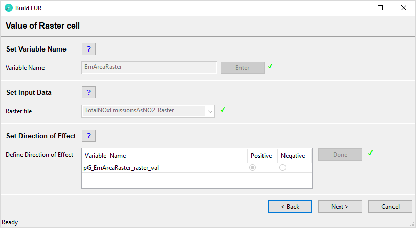
Click Next > to continue. The Predictors page will open again. You can scroll through the list under Predictors Added to check that you have added all potential predictors that you would like to analyse.

Click Next >.

Model

This is the final page of the Build LUR wizard. On this page you need to choose the type of model that you would like to build, before you finally build the model.

Export data (optional)
- Click the Export button. This will save the dependent variable and potential predictor variables in a text file. This file is formatted so that it can be read by most statistical software packages, which allows users with statistical expertise to run their own analyses on the data.
Build LUR model
- Under Type of model you can choose between building a classic model or a hybrid model. For the purpose of this tutorial select Classic LUR. For further information on the difference between classic and hybrid models click the help button or refer to the General Information section.
- Click Build model. Depending on the amount of data entered building the model may take several minutes.

The completed page should look like this:

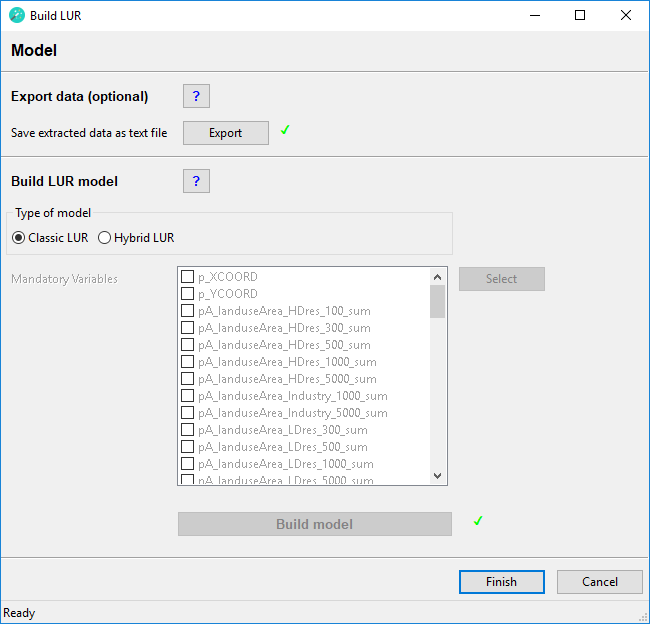
Click Finish.

Go to the directory of your output folder. Inside this folder you should see a new folder with the project name that you chose on the Settings page followed by a date and time stamp. Inside this new folder are the databases and files created by Build LUR:

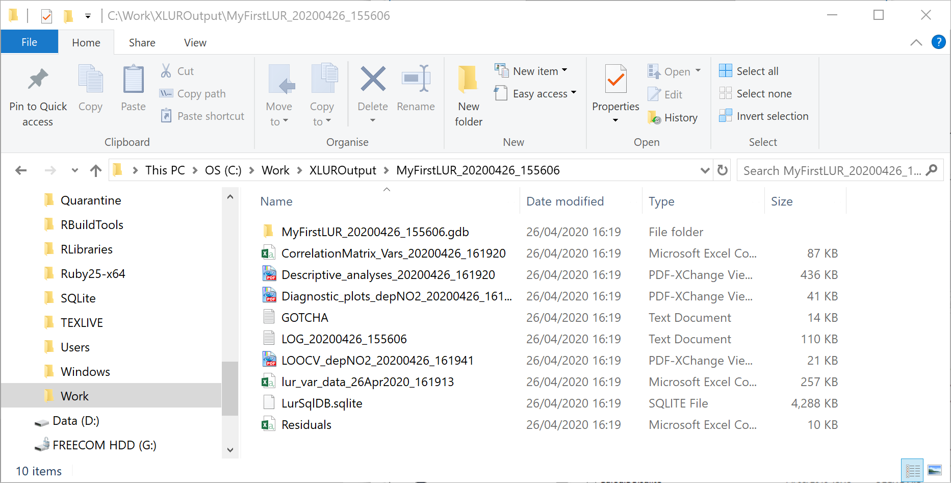
Click here for an overview of the files created in the Output folder.

Open the lur_var_data_[Date_Time].csv file. This is the text file that you exported on the Model page, which contains the dependent variable and all potential predictor variables. Scroll to the right and find the pD_EmissionAreaVal_NOxEmission_val variable and the pG_EmAreaRaster_raster_val variable. The values of these two variables are identical, which confirms that the value of nearest polygon and value of raster cell methods produced the same result when run on the same data.

Open the LOG_[Date_Time].txt file. This text file records all entries made into the Build LUR wizard, any warning or error messages, and the model development process. Scroll through this file until you find Predictor variables created. This lists all of the variables created through the Predictors pages of the wizard. You may notice that some variables are missing, e.g. pA_landuseArea_Port_100_sum is not there even though a buffer distance of 100 was specified for all land use categories. The missing variable is due to the fact that no Port land use area was found within any of the 100m buffers around the monitoring sites. Similarly, pC_EmissionPoint_Chemical_1000_sum, pC_EmissionPoint_Chemical_500_sum, pC_EmissionPoint_Chemical_300_sum, and pC_EmissionPoint_Chemical_100_sum are missing, because no point emission source from the chemical sector was present in the 1000m, 500m, 300m, or 100m buffers.

Scrolling down further through the file shows that a file of descriptive statistics was created in the output folder. This file shows the mean, median and variability of all dependent and predictor variables. If more than one dependent variable is selected this file will also show the correlation and pairwise regression plots of the dependent variables. This information can be useful to analyse the relationship between different pollutants. In this tutorial only one dependent variable was used, therefore these plots are empty. In addition, a correlation matrix of all variables was created and stored in the output folder. This can be helpful to identify variables that are highly correlated and therefore may be collinear in the regression model.

The next section shows details of the machine learning process used to develop the LUR model. XLUR uses supervised stepwise forward linear regression based on the methodology used in the ESCAPE study; see the General Information section for a brief overview of the variable selection process. XLUR records the starting model, all intermediate models (including reasons for their acceptance or rejection), and the final model. For the final model XLUR will also record the following model diagnostics in the log file:

Variance inflation factors - indicating the multicollinearity of the variables within the model
Case summaries and DF Betas - these can be used to check for bias in the model due to influential cases
Spatial autocorrelation of the residuals - based on Moran’s I, a large p-value indicates no spatial autocorrelation

Further model diagnostics are provided in Diagnostic_plots_dep[Outcome variable]_[Date_Time].pdf. This file shows a Q Q plot, which can be used to check the assumption of normality in the final model. It also shows a plot of the residuals vs the predicted values, which can be used to check for non-linear relationships, and a Scale-Location plot, which can be used to check for heteroscedasticity in the model.

XLUR will also carry out a leave one out cross validation of the final model, the results of which are shown in the LOOCV_[dependent variable name]_[Date_Time].pdf file. In a leave one out cross validation monitoring sites are removed one by one to test the performance of the final model. When a monitoring site is removed from the dataset the predictor variables of the final model are used to fit a new model, i.e. to calculate new coefficients, and this model is used to predict a value for the monitoring site that has been removed. This process is repeated for all monitoring sites and the measured and predicted values are plotted in a scatter plot. Using this scatterplot Pearson’s r, the adjusted R² and the Root Mean Squared Error (RMSE) are calculated.

For the purpose of this tutorial we will accept the final model and move on to the next step. However, it is recommended that users carefully check the model diagnostics when building their own models. If the model diagnostics indicate a problem, it may be necessary to manually develop a model using the lur_var_data_[Date_Time].csv file and standard statistical software.

The next step is to apply the LUR model created with the Build LUR wizard to unmeasured points within the study area.

Close and then restart ArcGIS Pro. (There is currently a known issue with ArcGIS Pro crashing, if XLUR is run multiple times, see the Troubleshooting section)
In the Catalog window double-click the ApplyLUR script.
In the Geoprocessing window on the right click Run. This will open the Apply LUR wizard.

Settings

Similar to the Build LUR wizard you need to specify some general settings on this page.

Set Output Name
- Next to Output Name type a suitable name for application output (e.g. LURApply) and click Enter.
Set Data Sources
- Click the Browse button next to LUR File Geodatabase. Navigate to the output directory that you used in the Build LUR wizard. In this directory select the MyFirstLUR_[Date_Time].gdb file geodatabase.
- Click the Browse button next to LUR SQLite Database. Navigate to the output directory that you used in the Build LUR wizard. In this directory select the LurSqlDB.sqlite database.
Set Model
- In the box next to Select LUR Model(s) tick MODEL_depNO2, then click Select.

The completed page should look like this:

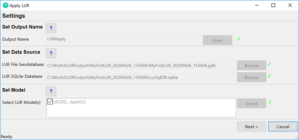
Click Next> to continue.

Receptors

To apply the LUR model to unmeasured locations within your study area you need to provide a number of receptor points. This page provides you with three options to do this: you can provide an existing point feature class, you can create regularly spaced points within your study area, or you can create a number of random points within your study area. For the purpose of this tutorial select B.Regular Points.

Receptors from Regular Points

On this page you need to specify the horizontal and vertical distance between points. The unit of the distance is the map unit of the projected coordinate system specified in the Build LUR wizard, which in this case is metres.

Set Distances
- In the box next to Horizontal Distance type 1000, then click Enter.
- In the box next to Vertical Distance type 1000, then click Enter.

The completed page should look like this:

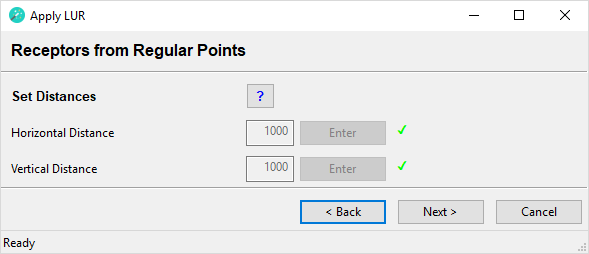
Click Next> to continue.

Apply Model

This is the final page of the Apply LUR wizard.

Apply LUR Model
- Click the Apply model button. Depending on the number of receptor points entered and the complexity of the model this may take a while.

The completed page should look like this:

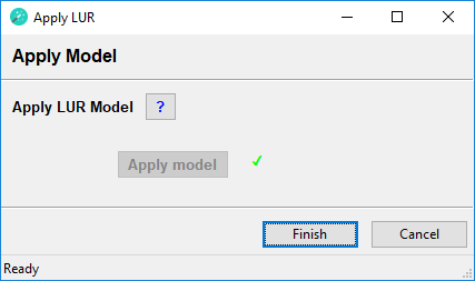
Click Finish to close the Apply LUR wizard.

Go to the directory of your output folder. Inside your MyFirstLUR_[Date_Time] folder you should see a new folder called LURApply_[DateTime]. Go inside this new folder. You should see two databases and two text files:

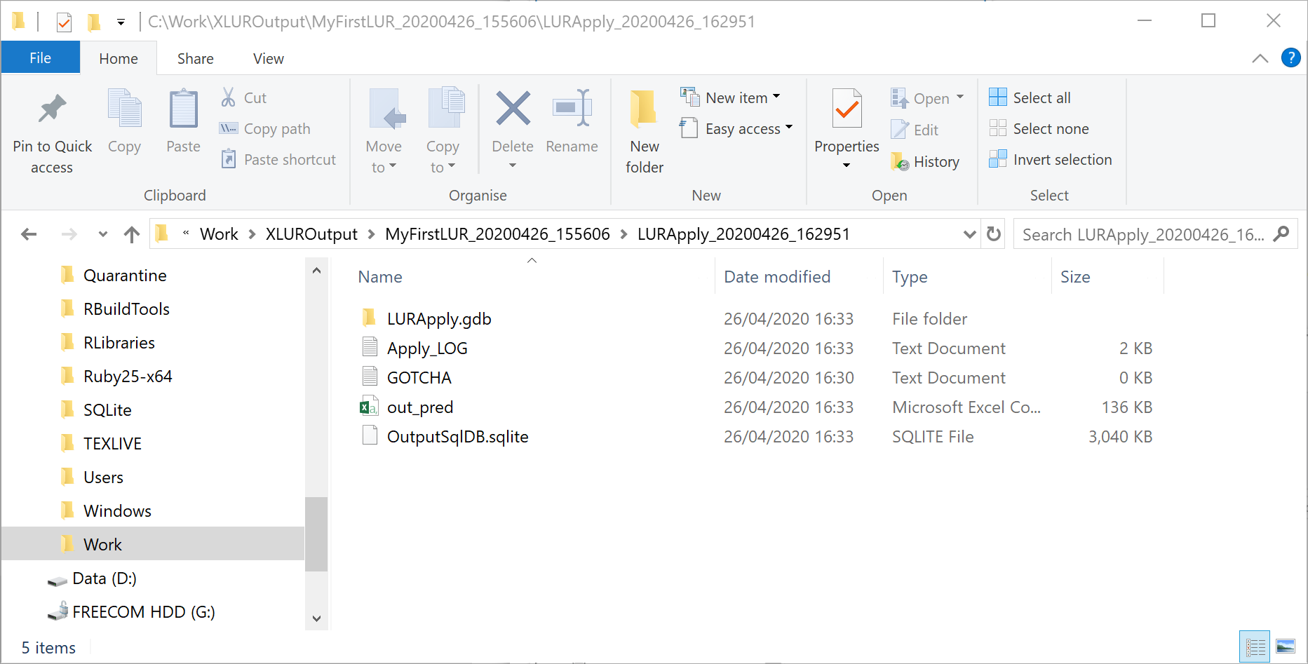
Open the Apply_Log.txt file. Similar to the Build LUR wizard this text file records all entries made into the Apply LUR wizard. In addition, it indicates the time it took to extract values for each predictor variable and to calculate predicted values.

The out_pred.csv file contains the coordinates of the receptor points, the values of the predictor variables at each receptor point and the predicted values of NO₂ at each receptor point. This data has also been added as a feature class to the LURApply file geodatabase. This enables the user to use the predicted values in further analyses or to report them as results on a map.

To quickly view the predicted values calculated by the Apply LUR wizard:

In ArcGIS Pro insert a new map.
Click on Add Data and navigate to the LURApply_[Date_Time] folder.
Open the LURApply.gdb file geodatabase, then open the LURdata feature dataset and select pred_lyr. The pred_lyr feature class contains predicted values for all dependent variables. In this case there was only one dependent variable, which was monitored NO₂.
In the Appearance menu click on Symbology and select the Graduated Colors option.
In the Symbology pane on the right select predNO2 in the dropdown list next to Field.
Select Quantile in the dropdown list next to Method.
Choose a suitable number for Classes (e.g. 5) and a suitable Color scheme (e.g. Prediction).

You should see something similar to this:

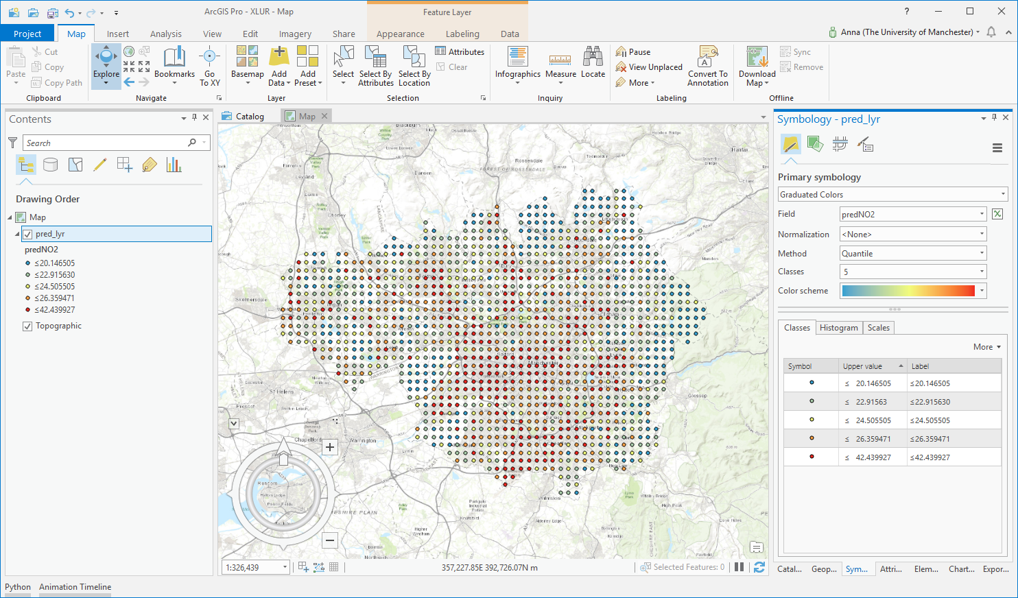
The TutorialOutput folder contains examples of the variable data, descriptive analyses, correlation matrix, diagnostic plots, log file, residuals, and leave one out crossvalidation plot created during the Build LUR step. The LURApply subfolder contains examples of the log file and output value file created during the Apply LUR step.

XLUR Wizard

v.2020-11-23

Installation

General Information

What is LUR?

The XLUR Wizard

Information Windows

Warning Windows

Error Windows

How does XLUR work?

Data Preparation

Study Area

Dependent Variable

Predictor Variables

Vector maps

Buffer based Predictors

Distance based Predictors

Raster maps

Build LUR

Step 1 - Settings

Set Project Name

Set Project Name

Project Name

Set Directories

Set Directories

Input File Geodatabase

Output Folder

Set Coordinate System

Set Coordinate System

Enter WKID number

Set Study Area

Set Study Area

Study Area Feature Class

Step 2 - Outcomes

Set Dependent Variable

Set Dependent Variable

Monitoring Sites

Select Site ID

Dependent Variables

Step 3 - Predictors

Buffer based Predictors

Polygon Area or Value within Buffer

Set Variable Name

Set Variable Name

Variable Name

Name Schema for Polygon Area or Value within Buffer

Set Buffer Sizes

Set Buffer Sizes

Buffers

Create Buffer Distance

Select Buffer Distance

Set Input Data

Set Input Data

Polygon Feature Class

Category Field

Aggregation Method

Value Field

Set Direction of Effect

Set Direction of Effect

Define Direction of Effect

Line Length or Value within Buffer

Set Variable Name

Set Variable Name

Variable Name

Name Schema for Line Length or Value within Buffer

Set Buffer Sizes

Set Buffer Sizes

Buffers

Create Buffer Distance

Select Buffer Distance

Set Input Data

Set Input Data

Line Feature Class

Category Field

Aggregation Method

Value Field

Set Direction of Effect

Set Direction of Effect

Define Direction of Effect

Point Count or Value within Buffer