Predictor variables can be derived from vector data and from raster data. From vector data predictor variables can be extracted based on circular buffers around the monitoring sites or based on the distance to the nearest feature. Since vector data can be polygons, lines or points, this results in six possible types of predictor variables. From raster data only the value of the raster cell that that is spatially coincident with the monitoring site point can be extracted, adding one more possible type of predictor. Therefore, in total seven types of predictor variables can be extracted and entered into the statistical analysis. Each type of variable can produce multiple predictors, depending on additional settings such as the number of buffer distances, the number of categories within a feature class, or the aggregation/extraction method specified.
For this type of variable a polygon feature class should be used, which has a spatial extent that is larger than that of the study area and the largest buffer distance. The polygon feature class should not contain duplicates or invalid geometries (if uncertain about invalid geometries, run the Check Geometry or Repair Geometry tool prior to running the wizard). The polygon feature class must contain a text field, which identifies a category for each polygon. If the feature class contains only one category of polygon, a dummy text field should be created with all rows set to the same value.
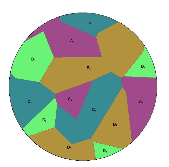
This example diagram is based on a polygon feature class with four categories (A,B,C,D). For a given buffer distance the wizard will calculate the total area (in the squared map unit of the projected coordinate system) of each category within the buffer, e.g.
A real life example of this variable type would be a polygon feature class of land use. Each category would contain a different type of land use, for example residential, industrial, commercial etc. Total land areas of each land use category within the circular buffer would be produced, e.g. in m2 for the British National Grid.
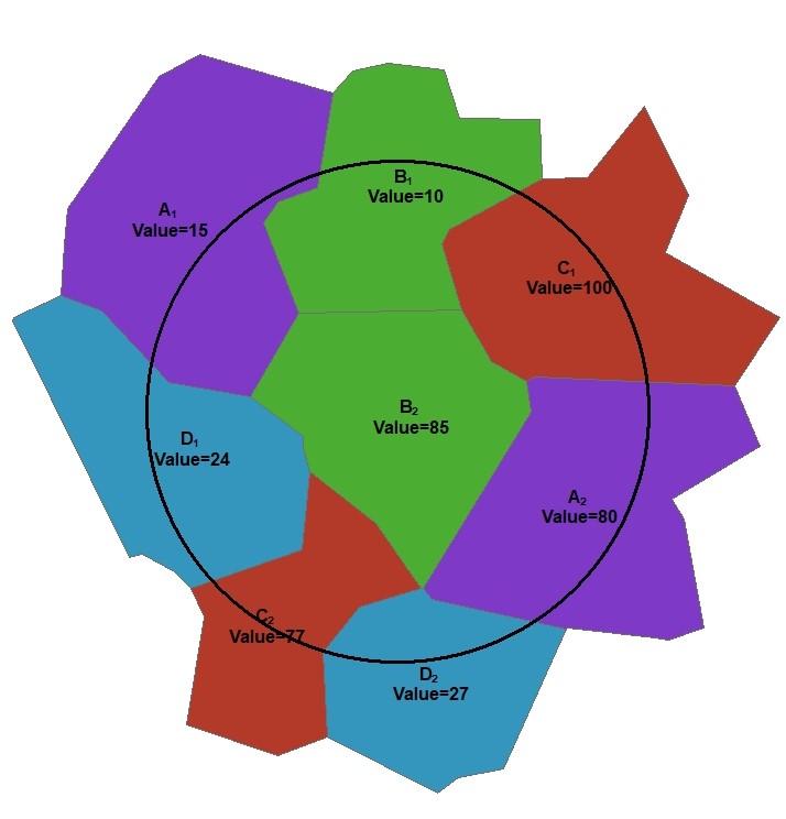
This example diagram is based on a polygon feature class with four categories (A,B,C,D) and each polygon has a numeric value attribute ("Value"). For a given buffer distance the wizard will calculate the total area weighted value for each category within the buffer, e.g.
A real life example of this variable type would be a polygon feature class of population density.
Alternatively, the wizard can calculate the total sum of the product of the polygon area and the polygon value, e.g.
A real life example of this variable type would be a polygon feature class of area emission sources such as fugitive emissions from land use categories based on different estimated car parking densities. Another example is anthropogenic heat emissions from different residential land uses depending on housing characteristics and estimated energy use.
Back to topFor this type of variable a line feature class should be used, which has a spatial extent that is larger than: the study area + the largest buffer distance. The line feature class should not contain duplicates. The line feature class must contain a text field, which identifies a category for each line. If the feature class contains only one category, a dummy text field should be created with all rows set to the same value.
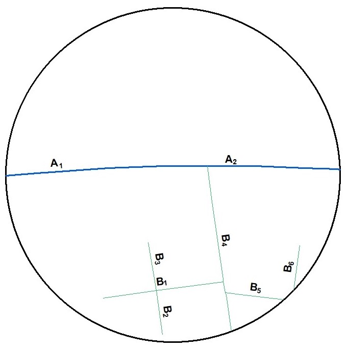
This example diagram is based on a line feature class with two categories (A,B). For a given buffer distance the wizard will calculate the total length (in the map unit of the projected coordinate system) of each category within the buffer, e.g.
A real life example of this variable type would be a line feature class of roads. Each category would contain a different type of road, for example motorway, local street etc. Total line lengths of each land use category within the circular buffer would be produced, e.g. in m for the British National Grid.
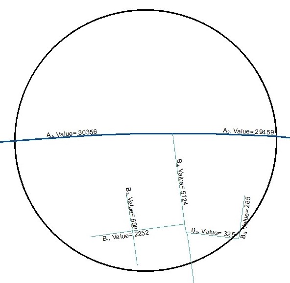
This example diagram is based on a line feature class with two categories (A,B) and each line has a numeric value. For a given buffer distance the wizard will calculate the total length weighted value for each category within the buffer, e.g.
A real life example of this variable type would be a line feature class of traffic counts.
Alternatively, the wizard can calculate the total sum of the product of the line length and the line value, e.g.
A real life example of this variable type would be a line feature class of proxy emissions loadings represented by average vehicle-kilometres per day.
Back to topFor this type of variable a point feature class should be used, which has a spatial extent that is larger than: the study area + the largest buffer distance. The point feature class should not contain duplicates. The point feature class must contain a text field, which identifies a category for each point. If the feature class contains only one category, a dummy text field should be created with all rows set to the same value.
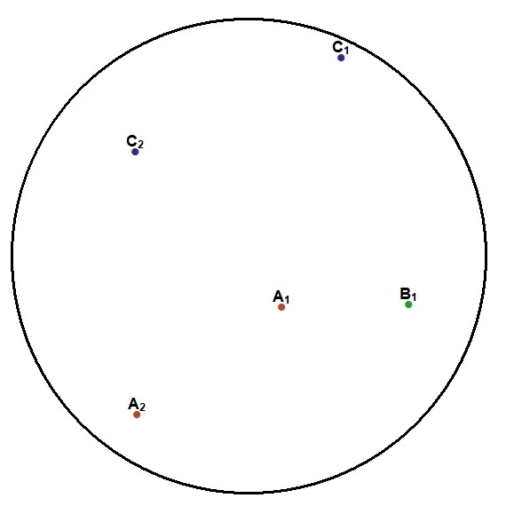
This example diagram is based on a point feature class with three categories (A,B,C). For a given buffer distance the wizard will count the number of points belonging to each category within the buffer, e.g.
A real life example of this variable type would be a point feature class of trees. Each category would contain a different tree species, for example Quercus robur, Fagus sylvatica, Cornus sanguinea etc. The count would therefore be the number of individuals of each species within the buffer. Another example would be the count of particular stacks (chimneys) used as a proxy of emission rates.
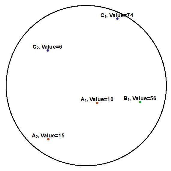
This example diagram is based on a point feature class with three categories (A,B,C) and each point has a numeric attribute value. For a given buffer distance the wizard will calculate the sum of values for each category within the buffer, e.g.
A real life example of this variable type would be a point feature class of chimney stacks with different emission rates (e.g. grammes of NOx per hour).
Alternatively, the wizard can calculate the mean or median of the values, e.g.
A real life example of this variable type would be tree height.
Back to topFor this type of variable a polygon feature class should be used, which ideally has a spatial extent that is larger than the study area. The polygon feature class must not contain spatial duplicates or invalid geometries (if uncertain about invalid geometries, run the Check Geometry or Repair Geometry tool prior to running the wizard).
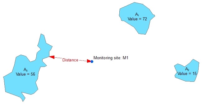
This example diagram shows a feature class of non-contiguous polygons with different values for each feature. For each each point feature representing a monitoring site the wizard will identify the nearest polygon and calculate one or more of the following options:
A real life example of this variable type would be proximity to water bodies with the potential to reduce air temperatures monitored at weather stations or the impact of fugitive emission sources from industrial sites on air quality. Inverse squared distance values are useful to represent the importance of distance, i.e. to give greater importance to nearby polygon features compared with those further away. A value attribute field might be useful if the size of the feature is important, e.g. livestock densities on agricultural land parcels in the case of ambient ammonia concentrations.
If the monitoring site is located on top of a polygon (i.e. the distance is zero) the Inverse distance, Inverse distance squared, Value * Inverse Distance, and Value * Inverse distance squared options will produce a division by zero error and the result for the feature will be set to missing. The Distance and Value * Distance options will produce a result of zero. Therefore, the user should carefully inspect the data prior to using these options.
Back to topFor this type of variable a line feature class should be used, which ideally has a spatial extent that is larger than the study area. The line feature class must not contain spatial duplicates.
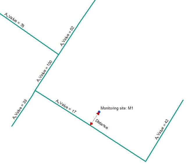
This example diagram shows a line feature class with different values for each feature. For each point feature representing a monitoring site loaction the wizard will identify the nearest line and calculate one or more of the following options:
A real life example of this variable type would be proximity to the nearest road feature to represent the potential for higher ambient air pollutant concentrations due to vehicular emissions or proximity to the nearest river to represent the potential for lower air temperatures at nearby weather stations. Inverse squared distance values are useful to represent the importance of distance, i.e. to give greater importance to nearby line features compared with those further away. A Value attribute field might be useful if the size of the feature is important, e.g. roads with an attribute representing traffic volume.
If the monitoring site is located on top of a line (i.e. the distance is zero) the Inverse distance, Inverse distance squared, Value * Inverse Distance, and Value * Inverse distance squared options will produce a division by zero error and the result for the feature will be set to missing. The Distance and Value * Distance options will produce a result of zero. Therefore, the user should carefully inspect the data prior to using these options.
Back to topFor this type of variable a point feature class should be used, which ideally has a spatial extent that is larger than the study area. The point feature class must not contain spatial duplicates.
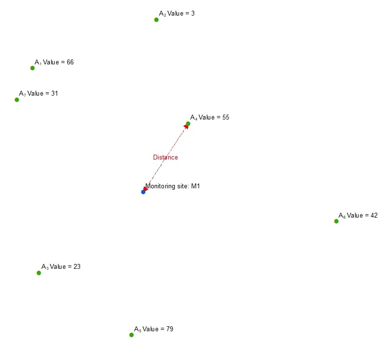
This example diagram shows a point feature class with different values for each feature. For each monitoring site the wizard will identify the nearest point and calculate one or more of the following options:
A real life example of this variable type would be proximity to the nearest point feature representing a chimney stack. In this case closer distances are more likely to result in higher pollutant concentrations. Inverse squared distance values are useful to represent the importance of distance, i.e. to give greater importance to nearby point features compared with those further away. A Value attribute field might be useful if the size of the feature is important, e.g. the emission rate from the chimney stack.
If the monitoring site is located on top of a point (i.e. the distance is zero) the Inverse distance, Inverse distance squared, Value * Inverse Distance, and Value * Inverse distance squared options will produce a division by zero error and the result for the feature will be set to missing. The Distance and Value * Distance options will produce a result of zero. Therefore, the user should carefully inspect the data prior to using these options.
Back to topFor this type of variable a raster grid file should be used, which ideally has a spatial extent that is larger than the study area. The wizard will extract the value of the raster cell that is spatially coincident with the point location representing the monitoring site (dependent variable).
An example of the use of this predictor variable type is elevation. Elevation is commonly sourced from a Digital Elevation Model stored as a raster grid.
Back to top